![]()
Table of Contents
The goal of AdmixPoly is to provide functions to perform global and local admixture inference from bi- and multi-allelic marker dosages (discrete or continuous) in polyploid species.
You can install AdmixPoly directly from the CRAN (not available at the moment):
install.packages(pkg='AdmixPoly',repos='https://cran.r-project.org/')or from the source repository (GitLab) using remotes:
install.packages(pkg='remotes', repos='https://cran.r-project.org/')
remotes::install_git('https://gitlab.cirad.fr/agap/seg/admixpoly.git')
When installing from the GitLab repository, first make sure to have a compilation environment installed on your system.
Windows (≥ 10)
Download and install the appropriate 64-bits version of Rtools and git.
GNU/Linux. Depending on your distribution run one of the commands below.
Debian and derivative (e.g. Ubuntu, Mint):
apt-get install g++ git libicu-devRedhat and derivative (e.g. Fedora, Centos, RockyLinux):
dnf install gcc-c++ git libicu-develmacOS
Check if git and the clang compiler are installed with these commands in a terminal window:
clang --version
git --version
If not, run this command:
xcode-select --installThis is a basic example illustrating how to perform admixture inference using AdmixPoly.
First, an admixed dataset is simulated using the
SimulatePop function, considering N=100
individuals of ploidy P=8, M=1000 markers with
L=10 alleles distributed on C=5 chromosomes,
and K=4 ancestral groups.
DataSim <- AdmixPoly::SimulatePop(K=3L, N=100L, P=8L, M=1000L, C=2L, L=10L)The resulting DataSim object includes:
Geno: list of genotyping matrices over markershead(DataSim$Geno[[1]])
#> Allele1 Allele2 Allele3 Allele4 Allele5 Allele6 Allele7 Allele8 Allele9
#> Ind1 0 1 0 0 1 1 1 0 1
#> Ind2 0 2 3 0 1 0 1 0 0
#> Ind3 0 5 2 0 0 0 1 0 0
#> Ind4 0 1 2 2 0 0 1 2 0
#> Ind5 0 3 1 1 0 0 2 0 0
#> Ind6 0 1 1 1 1 2 1 1 0
#> Allele10
#> Ind1 3
#> Ind2 1
#> Ind3 0
#> Ind4 0
#> Ind5 1
#> Ind6 0Prop: matrix of admixture proportionshead(DataSim$Prop)
#> K1 K2 K3
#> Ind1 0.106375 0.431750 0.461875
#> Ind2 0.587625 0.394000 0.018375
#> Ind3 0.680500 0.217500 0.102000
#> Ind4 0.509500 0.490500 0.000000
#> Ind5 0.859500 0.033125 0.107375
#> Ind6 0.181125 0.267750 0.551125Freq: list of matrices of allele frequencies in
ancestral groupsDataSim$Freq[[1]]
#> Allele1 Allele2 Allele3 Allele4 Allele5 Allele6 Allele7
#> K1 0.02999937 0.3216599409 0.2827303 0.06252135 0.04569980 0.01259175 0.1560145
#> K2 0.06062462 0.0007481235 0.3483231 0.01478613 0.04326888 0.04442491 0.1591765
#> K3 0.00337067 0.0736675715 0.3034438 0.06786697 0.17255898 0.11904414 0.1678521
#> Allele8 Allele9 Allele10
#> K1 0.01215938 0.019408693 0.05721497
#> K2 0.19739411 0.001450772 0.12980285
#> K3 0.03792193 0.036377344 0.01789647GeneticMap: genetic map dataframehead(DataSim$GeneticMap)
#> Marker Chromosome Distance
#> 1 Marker1 Chr1 0.0000000
#> 2 Marker2 Chr1 0.2004008
#> 3 Marker3 Chr1 0.4008016
#> 4 Marker4 Chr1 0.6012024
#> 5 Marker5 Chr1 0.8016032
#> 6 Marker6 Chr1 1.0020040From simulated data, admixture proportions can be estimated using the
AdmixGlobal function:
ResGlobalAdmix <- AdmixPoly::AdmixGlobal(Geno=DataSim$Geno, K=3L,MaxIter=1000,Verbose=F)The estimated admixture proportions are available from:
head(ResGlobalAdmix$Prop)
#>              K1         K2         K3
#> Ind1 0.42751014 0.09196272 0.48052714
#> Ind2 0.39607077 0.60392823 0.00000100
#> Ind3 0.18982802 0.71856785 0.09160413
#> Ind4 0.47932675 0.52067225 0.00000100
#> Ind5 0.01352721 0.92827717 0.05819562
#> Ind6 0.24174073 0.19640609 0.56185317
They can be represented using the ggplot2-based
GlobalPlot function:
AdmixPoly::GlobalPlot(ResGlobalAdmix$Prop)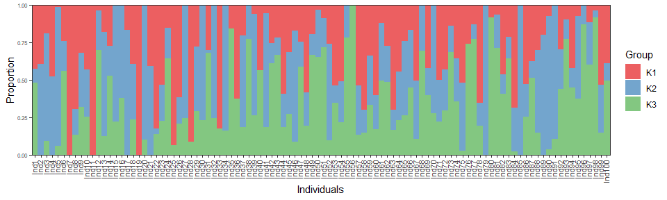
Estimated proportions are very close to simulated ones (up to an arbitrary labeling of groups), as indicated by the root mean square error (RMSE):
group_corresp <- apply(cor(DataSim$Prop,ResGlobalAdmix$Prop),2,which.max)
sqrt(mean((DataSim$Prop-ResGlobalAdmix$Prop[,group_corresp])^2))
#> [1] 0.02168584
Estimated allele frequencies are available from:
ResGlobalAdmix$Freq[[1]]
#>       Allele1    Allele2   Allele3    Allele4    Allele5    Allele6   Allele7
#> K1 0.06565551 0.00000100 0.3477740 0.00000100 0.03057859 0.06962224 0.1208821
#> K2 0.03109042 0.29182439 0.2713478 0.06719518 0.07038353 0.01340646 0.1872236
#> K3 0.00000100 0.05668937 0.2049396 0.07104907 0.13114363 0.14552308 0.2449462
#>       Allele8     Allele9   Allele10
#> K1 0.19902928 0.000001000 0.16645533
#> K2 0.00000100 0.009649829 0.05787779
#> K3 0.06641198 0.034075409 0.04522066
The convergence can be checked from the log-likelihood:
plot(ResGlobalAdmix$LogLik, xlab="Iterations", ylab="LogLik", type="o")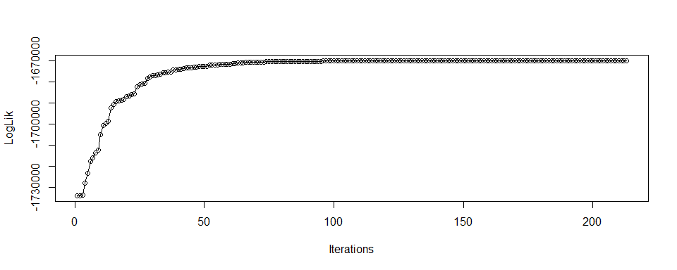
Let us consider a second admixed population from the same ancestral groups with a higher admixture level by specifying a higher ‘AlphaProp’ value.
DataSim2 <- AdmixPoly::SimulatePop(K=3L, N=100L, P=8L, M=1000L, C=2L, L=10L,
                                   AlphaProp = 10, Freq = DataSim$Freq)
The higher admixture level can be illustrated using a barplot of simulated amdixture proportions.
AdmixPoly::GlobalPlot(DataSim2$Prop)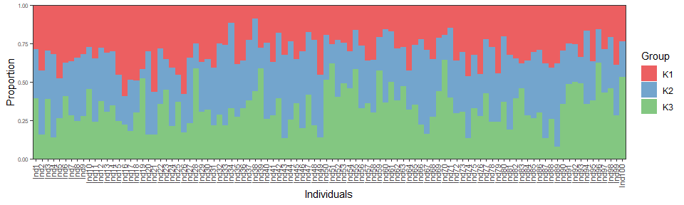
In this case, it can be beneficial to initialize the algorithm with ancestral allele frequencies estimated using the first population ‘FreqInit=ResGlobalAdmix$Freq’ and only update admixture proportions ‘ParamToUpdate=“Prop”’.
ResGlobalAdmix2 <- AdmixPoly::AdmixGlobal(Geno=DataSim2$Geno, K=3L, MaxIter=1000, Verbose=F,
                                          FreqInit=ResGlobalAdmix$Freq, ParamToUpdate="Prop")
Again, estimated proportions are very close to simulated ones, as indicated by the RMSE:
sqrt(mean((DataSim2$Prop-ResGlobalAdmix2$Prop[,group_corresp])^2))
#> [1] 0.02526292Based on global admixture results, local admixture can be estimated
for a given individual using the AdmixLocal function:
Ind <- "Ind3"
ResLocalAdmix <- AdmixPoly::AdmixLocal(Geno=DataSim$Geno,ResAdmixGlobal = ResGlobalAdmix,
                                       GeneticMap = DataSim$GeneticMap,Ind = Ind,P = 8L,
                                       SmoothParam = 1,Verbose=F)
Local ancestry dosages based on posterior probabilities are available from:
head(ResLocalAdmix$Posterior$Chr1)
#>                 K1       K2       K3
#> Marker1 0.02838614 6.966770 1.004844
#> Marker2 0.02683719 6.966129 1.007034
#> Marker3 0.02464581 6.965626 1.009728
#> Marker4 0.02337629 6.966975 1.009649
#> Marker5 0.02250143 6.968826 1.008673
#> Marker6 0.02199903 6.970135 1.007866
Alternatively, local ancestry dosages based on the Viterbi algorithm are available from:
head(ResLocalAdmix$Viterbi$Chr1)
#>         K1 K2 K3
#> Marker1  0  7  1
#> Marker2  0  7  1
#> Marker3  0  7  1
#> Marker4  0  7  1
#> Marker5  0  7  1
#> Marker6  0  7  1
The RMSE of estimated local ancestry proportions (ancestry dosages divided by the ploidy) is:
sqrt(mean((DataSim$Ancestry[[Ind]]$Chr1/8-ResLocalAdmix$Posterior$Chr1[,group_corresp]/8)^2))
#> [1] 0.01208612
sqrt(mean((DataSim$Ancestry[[Ind]]$Chr1/8-ResLocalAdmix$Viterbi$Chr1[,group_corresp]/8)^2))
#> [1] 0.01118034
Local ancestry dosages can be represented using the ggplot2-based
LocalPlot function:
AdmixPoly::LocalPlot(Ancestry = ResLocalAdmix$Posterior, GeneticMap = DataSim$GeneticMap)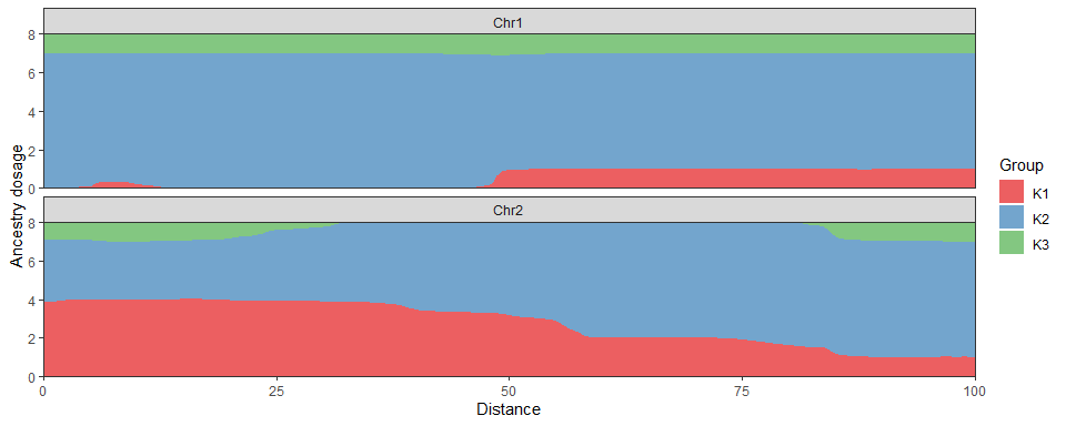
Local admixture inference over the five first individuals can be run using:
ResLocalAdmix_list <- lapply(paste0("Ind",1:5),function(i){
  res_i <- AdmixPoly::AdmixLocal(Geno=DataSim$Geno,ResAdmixGlobal = ResGlobalAdmix,
                               GeneticMap = DataSim$GeneticMap,Ind = i,P = 8L,
                               SmoothParam = 1,Verbose=F)
  return(res_i)
})
When computing time is large, each individual can be run in parallel on a high-performance computing cluster.
Genotyping data formatted as a variant call format (VCF) can be imported as:
vcf_path <- system.file("extdata", "Test.vcf", package = "AdmixPoly")
DataVCF <- AdmixPoly::ReadVCF(File = vcf_path)
The resulting DataVCF object includes:
MarkerInfo: first eight columns of the VCFhead(DataVCF$MarkerInfo)
#> # A tibble: 6 × 9
#> MARKER CHROM POS ID REF ALT QUAL FILTER INFO
#> <chr> <chr> <int> <chr> <chr> <chr> <chr> <chr> <chr>
#> 1 Chr1_15892318 Chr1 15892318 . A T . . .
#> 2 Chr1_31209423 Chr1 31209423 . T C . . .
#> 3 Chr1_39962954 Chr1 39962954 . C G . . .
#> 4 Chr1_40515463 Chr1 40515463 . G A . . .
#> 5 Chr1_44904209 Chr1 44904209 . A T . . .
#> 6 Chr1_47542399 Chr1 47542399 . T C . . .Geno: list of genotyping matriceshead(DataVCF$Geno[[1]])
#> A T
#> IND1 4 4
#> IND2 5 3
#> IND3 1 7
#> IND4 4 4
#> IND5 0 8
#> IND6 4 4GeneticMap: genetic map dataframe in which physical
between first and last marker of each chromosome are scaled to 100
cMhead(DataVCF$GeneticMap)
#> # A tibble: 6 × 3
#> Chromosome Marker Distance
#> <chr> <chr> <dbl>
#> 1 Chr1 Chr1_15892318 0
#> 2 Chr1 Chr1_31209423 20.4
#> 3 Chr1 Chr1_39962954 32.1
#> 4 Chr1 Chr1_40515463 32.9
#> 5 Chr1 Chr1_44904209 38.7
#> 6 Chr1 Chr1_47542399 42.2Instead of estimated dosages, read depth ratios can be imported by specifying the allele read depths field of the FORMAT column:
DataVCF2 <- AdmixPoly::ReadVCF(File = vcf_path,AlleleDepthField = "AD")head(DataVCF2$Geno[[1]])
#> A T
#> IND1 0.41935484 0.5806452
#> IND2 0.50000000 0.5000000
#> IND3 0.08108108 0.9189189
#> IND4 0.68181818 0.3181818
#> IND5 0.03125000 0.9687500
#> IND6 0.53125000 0.4687500Please note that read depth ratios are not scaled to the ploidy level, which must then be informed in the inference functions.
Another function can be used to read the haplotype presence-absence (HPA) format obtained from HaploCharmer:
hpa_path <- system.file("extdata", "Test.hpa", package = "AdmixPoly")
DataHPA <- AdmixPoly::ReadHPA(File = hpa_path)head(DataHPA$Geno[[1]])
#> hap1 hap2 hap3
#> IND1 0.54545455 0.1818182 0.2727273
#> IND2 0.48888889 0.2444444 0.2666667
#> IND3 0.08823529 0.6764706 0.2352941
#> IND4 0.08108108 0.4054054 0.5135135
#> IND5 0.00000000 0.3684211 0.6315789
#> IND6 0.45454545 0.1818182 0.3636364