The goal of CohortSymmetry is to carry out the necessary calculations for Sequence Symmetry Analysis (SSA). It is highly recommended that this method is tested beforehand against well-known positive and negative controls. Such controls could be found using Pratt et al (2015).
You can install the development version of CohortSymmetry from GitHub with:
# install.packages("devtools")
devtools::install_github("OHDSI/CohortSymmetry")The CohortSymmetry package is designed to work with data in the OMOP
CDM (Common Data Model) format, so our first step is to create a
reference to the data using the CDMConnector package.
As an example, we will be using Eunomia data set.
library(CDMConnector)
library(dplyr)
library(DBI)
library(duckdb)

db <- DBI::dbConnect(duckdb::duckdb(),
                     dbdir = CDMConnector::eunomiaDir())
cdm <- cdmFromCon(
  con = db,
  cdmSchema = "main",
  writeSchema = "main"
)This will be entirely user’s choice on how to generate such cohorts. Minimally, this package requires two cohort tables in the cdm reference, namely the index_cohort and the marker_cohort.
If one wants to generate two drugs cohorts in cdm, DrugUtilisation is recommended. For merely illustration purposes, we will carry out PSSA on aspirin (index_cohort) against amoxicillin (marker_cohort)
library(dplyr)
library(DrugUtilisation)
cdm <- DrugUtilisation::generateIngredientCohortSet(
  cdm = cdm,
  name = "aspirin",
  ingredient = "aspirin")
#> ℹ Subsetting drug_exposure table
#> ℹ Checking whether any record needs to be dropped.
#> ℹ Collapsing overlaping records.
#> ℹ Collapsing records with gapEra = 1 days.

cdm <- DrugUtilisation::generateIngredientCohortSet(
  cdm = cdm,
  name = "amoxicillin",
  ingredient = "amoxicillin")
#> ℹ Subsetting drug_exposure table
#> ℹ Checking whether any record needs to be dropped.
#> ℹ Collapsing overlaping records.
#> ℹ Collapsing records with gapEra = 1 days.In order to initiate the calculations, the two cohorts tables need to
be intersected using generateSequenceCohortSet(). This
process will output all the individuals who appeared on both tables
according to a user-specified parameters. This includes
timeGap, washoutWindow,
indexMarkerGap and daysPriorObservation.
Details on these parameters could be found on the vignette.
library(CohortSymmetry)

cdm <- generateSequenceCohortSet(
  cdm = cdm,
  indexTable = "aspirin",
  markerTable = "amoxicillin",
  name = "aspirin_amoxicillin"
)

cdm$aspirin_amoxicillin %>%
  dplyr::glimpse()
#> Rows: ??
#> Columns: 6
#> Database: DuckDB v1.1.3 [xihangc@Windows 10 x64:R 4.2.1/C:\Users\xihangc\AppData\Local\Temp\Rtmpy2oj4K\file791c79b03ba9.duckdb]
#> $ cohort_definition_id <int> 1, 1, 1, 1, 1, 1, 1, 1, 1, 1, 1, 1, 1, 1, 1, 1, 1…
#> $ subject_id           <int> 563, 1669, 2141, 3145, 3440, 4052, 4776, 331, 161…
#> $ cohort_start_date    <date> 1964-06-11, 1959-12-29, 1950-06-23, 1974-11-14, …
#> $ cohort_end_date      <date> 1964-08-16, 1960-02-05, 1950-11-14, 1975-04-06, …
#> $ index_date           <date> 1964-06-11, 1959-12-29, 1950-11-14, 1975-04-06, …
#> $ marker_date <date> 1964-08-16, 1960-02-05, 1950-06-23, 1974-11-14, …To get the sequence ratios, we would need the output of the
generateSequenceCohortSet() function to be fed into
summariseSequenceRatios() The output of this process
contains cSR(crude sequence ratio), aSR(adjusted sequence ratio) and
confidence intervals.
res <- summariseSequenceRatios(cohort = cdm$aspirin_amoxicillin)

res %>% glimpse()
#> Rows: 10
#> Columns: 13
#> $ result_id        <int> 1, 1, 1, 1, 1, 1, 1, 1, 1, 1
#> $ cdm_name         <chr> "An OMOP CDM database", "An OMOP CDM database", "An O…
#> $ group_name       <chr> "index_cohort_name &&& marker_cohort_name", "index_co…
#> $ group_level      <chr> "aspirin &&& amoxicillin", "aspirin &&& amoxicillin",…
#> $ strata_name      <chr> "overall", "overall", "overall", "overall", "overall"…
#> $ strata_level     <chr> "overall", "overall", "overall", "overall", "overall"…
#> $ variable_name    <chr> "crude", "adjusted", "crude", "crude", "adjusted", "a…
#> $ variable_level   <chr> "sequence_ratio", "sequence_ratio", "sequence_ratio",…
#> $ estimate_name    <chr> "point_estimate", "point_estimate", "lower_CI", "uppe…
#> $ estimate_type    <chr> "numeric", "numeric", "numeric", "numeric", "numeric"…
#> $ estimate_value   <chr> "1.43589743589744", "1629.5148627184", "0.95731197561…
#> $ additional_name  <chr> "overall", "overall", "overall", "overall", "overall"…
#> $ additional_level <chr> "overall", "overall", "overall", "overall", "overall"…The user could then visualise their results using a wide array of provided tools.
For example, the following produces a gt table.
gt_results <- tableSequenceRatios(result = res)
gt_results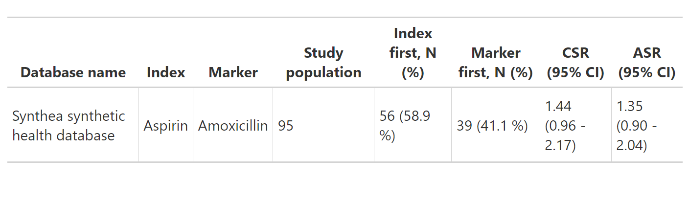 Note that flextable
is also an option, users may specify this by using the
Note that flextable
is also an option, users may specify this by using the type
argument.
One could also visualise the plot, for example, the following is the plot of the adjusted sequence ratio.
plotSequenceRatios(result = res,
                  onlyaSR = T,
                  colours = "black")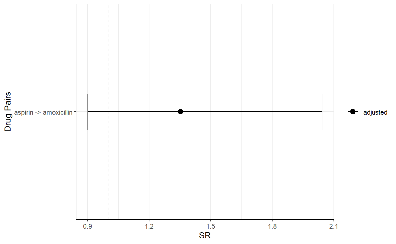
The user also has the freedom to plot temporal trend like so:
plotTemporalSymmetry(cdm = cdm, sequenceTable = "aspirin_amoxicillin")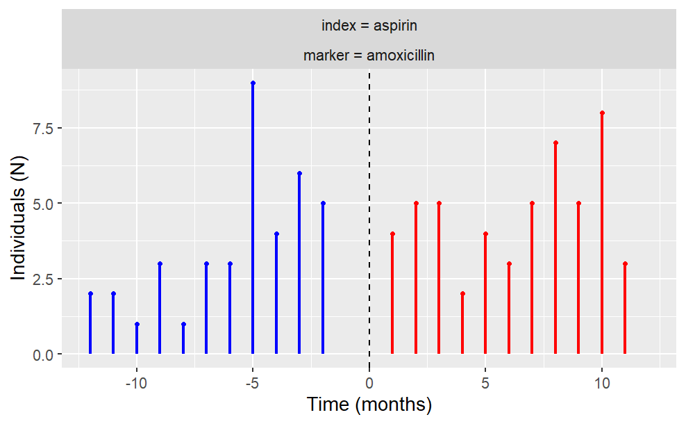
CDMConnector::cdmDisconnect(cdm = cdm)