The GPpenalty package in R provides maximum likelihood
estimation for Gaussian processes, supporting both isotropic and
separable models with predictive capabilities. Includes penalized
likelihood estimation using decorrelated prediction error (DPE)-based
metrics, motivated by Mahalanobis distance, that account for
uncertainty. Includes cross validation techniques for tuning parameter
selection. Designed specifically for small datasets.
You can install the development version of GPpenalty like so:
install.packages("GPpenalty")This is a basic example which shows you how to solve a common problem:
library(GPpenalty)
#>
#> Attaching package: 'GPpenalty'
#> The following object is masked from 'package:stats':
#>
#>     kernel
# one dimensional function
f_x <- function(x) {
  return(sin(2*pi*x) + x^2)
}
Generate training and testing data.
n <- 6
n.test <- 100
x <- matrix(seq(0, 1, length=n), ncol=1)
y <- f_x(x)
x.test <- matrix(seq(0, 1, length=n.test), ncol=1)
y.test <- f_x(x.test)
# center and standardize response
y.test <- (y.test-mean(y))/sd(y)
y <- (y-mean(y))/sd(y)
# scale x
x.min <- apply(x, 2, range)[1,]
x.max <- apply(x, 2, range)[2,]
x <- (x - x.min)/(x.max-x.min)
x.test <- (x.test - x.min)/(x.max-x.min)
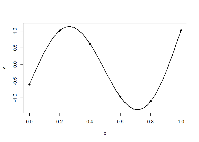
plot(x.test, y.test, type="l", xlab="x", ylab="y", lwd=2)
points(x, y, pch=19)
The black line is the true function and black dots represent the observed points.
Now fit a model and use the MLE value as a plug in estimator for prediction.
fit <- mle_gp(y, x)
p <- predict_gp(fit, x.test)
q1 <- p$mup - qnorm(0.025)*sqrt(diag(p$Sigmap))
q3 <- p$mup + qnorm(0.025)*sqrt(diag(p$Sigmap))

plot(x.test, y.test, type="l", xlab="x", ylab="y", lwd=2, ylim=range(q1, q3))
polygon(c(x.test, rev(x.test)), c(q1-0.04, rev(q3+0.04)),
        col = rgb(0.7, 0.7, 0.7, 0.5), border = NA)
points(x, y, pch=19)
lines(x.test, y.test, lwd = 4, col = 1)
lines(x.test, p$mup, lwd = 4, col = "blue", lty = 2)
points(x, y, pch = 19, cex = 2)
legend("bottomleft", legend = c("truth", "observed", "GP mean", "GP 95% CI"),
       lty = c(1, NA, 2, NA), col = c("black", "black", "blue", "gray"),
       lwd = c(3, NA, 3, NA), pch = c(NA, 19, NA, 15), pt.cex = 1.2,
       cex = 1,bty = "o", bg = "white")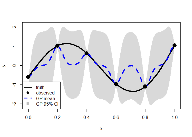
The blue dashed line represents the predictive mean function and the gray shaded area indicates the 95% CI. The CI appears inflated, and the predictive mean function shows poor performance.
We are going to penalize the lengthscale parameter, theta.
set.seed(0)
# k-fold cross validation
# dpe metric
cv <- gp_cv(y, x, k=3)
pmle <- mle_penalty(cv)
penalized.p <- predict_gp(pmle, x.test)

q1 <- penalized.p$mup - qnorm(0.025)*sqrt(diag(penalized.p$Sigmap))
q3 <- penalized.p$mup + qnorm(0.025)*sqrt(diag(penalized.p$Sigmap))

plot(x.test, y.test, type="l", xlab="x", ylab="y", lwd=2, ylim=range(q1, q3))
polygon(c(x.test, rev(x.test)), c(q1-0.04, rev(q3+0.04)),
        col = rgb(0.7, 0.7, 0.7, 0.5), border = NA)
points(x, y, pch=19)
lines(x.test, y.test, lwd = 4, col = 1)
lines(x.test, penalized.p$mup, lwd = 4, col = "blue", lty = 2)
points(x, y, pch = 19, cex = 2)
legend("bottomleft", legend = c("truth", "observed", "GP mean", "GP 95% CI"),
       lty = c(1, NA, 2, NA), col = c("black", "black", "blue", "gray"),
       lwd = c(3, NA, 3, NA), pch = c(NA, 19, NA, 15), pt.cex = 1.2,
       cex = 1,bty = "o", bg = "white")
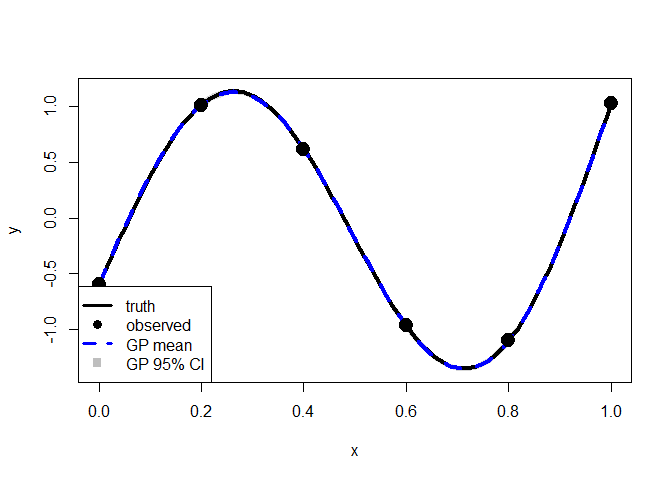
The tuning parameter, lambda, that minimizes the decorrelated prediction error (DPE) reverts to the MLE. To encourage additional shrinkage, we apply the one‑standard‑error rule.
pmle <- mle_penalty(cv, one.se = TRUE)
penalized.p <- predict_gp(pmle, x.test)

q1 <- penalized.p$mup - qnorm(0.025)*sqrt(diag(penalized.p$Sigmap))
q3 <- penalized.p$mup + qnorm(0.025)*sqrt(diag(penalized.p$Sigmap))

plot(x.test, y.test, type="l", xlab="x", ylab="y", lwd=2, ylim=range(q1, q3))
polygon(c(x.test, rev(x.test)), c(q1-0.04, rev(q3+0.04)),
        col = rgb(0.7, 0.7, 0.7, 0.5), border = NA)
points(x, y, pch=19)
lines(x.test, y.test, lwd = 4, col = 1)
lines(x.test, penalized.p$mup, lwd = 4, col = "blue", lty = 2)
points(x, y, pch = 19, cex = 2)
legend("bottomleft", legend = c("truth", "observed", "GP mean", "GP 95% CI"),
       lty = c(1, NA, 2, NA), col = c("black", "black", "blue", "gray"),
       lwd = c(3, NA, 3, NA), pch = c(NA, 19, NA, 15), pt.cex = 1.2,
       cex = 1,bty = "o", bg = "white")