



{colleyRstats}:
Functions to Streamline Statistical Analysis and ReportingCreated by Mark Colley
| Status | Usage | Miscellaneous |
|---|---|---|
|
|
|
|
|
colleyRstats is a collection of custom R functions that
streamline statistical analysis and result reporting. Built upon popular
R packages such as ggstatsplot and
ARTool, this collection
offers a wide array of tools for simplifying reproducible analyses,
generating high-quality visualizations, and producing APA-compliant
outputs.
The primary goal of this package is to significantly reduce
repetitive coding efforts, allowing you to focus on interpreting
results. Whether you’re dealing with ANOVA assumptions, reporting effect
sizes, or creating publication-ready visualizations,
colleyRstats makes these tasks easier.
score_questionnaire() applies a published instrument’s own
scoring key – NASA-TLX, SUS, UEQ / UEQ-S, TiA, AttrakDiff, IPQ, SSQ,
FMS, MISC – and check_questionnaire() shows the item
mapping before you trust the numbers.fit_recommended() carries recommend_test()
through to a fitted model, its post-hoc contrasts, and the manuscript
sentence, so the test you justify and the model you ran cannot drift
apart.use_study_project() scaffolds the whole analysis as a
targets pipeline with renv pinning, a Quarto
report, and generated LaTeX the manuscript \input{}s.ggstatsplot Wrappers:
Automatically switch between parametric and non-parametric versions of
tests based on the data’s characteristics.recommend_test() inspects your data (scale, clustering,
assumptions) and recommends the matching model – including mixed models
– with a ready-to-edit fit call and methods sentence.analyze_and_report() / report_all() produce
the figure, methods sentence, omnibus result, and post-hoc comparisons
for one or many dependent variables in a single call;
emit_overleaf() bundles everything into an Overleaf-ready
folder.save_paper_figure() saves them with publication
presets.| Type | Command |
|---|---|
| Release | install.packages("colleyRstats") |
| Development | remotes::install_github("M-Colley/colleyRstats") |
The vignettes walk through the main workflows end-to-end:
vignette("getting-started", package = "colleyRstats") –
setup, assumption checks, plotting, and reporting in a nutshell.vignette("analyzing-a-user-study", package = "colleyRstats")
– a typical (HCI) user study from raw data to manuscript-ready text and
figures.vignette("choosing-a-test", package = "colleyRstats") –
how recommend_test() selects tests and mixed models, and
how to report them.vignette("overleaf", package = "colleyRstats") –
getting the LaTeX output into an Overleaf project that compiles
immediately.The quickest way to see what the package does is the one-call pipeline:
library(colleyRstats)

result <- analyze_and_report(mtcars, dv = "mpg", iv = "cyl")
result$plot       # ggstatsplot figure (parametric/non-parametric auto-selected)
result$sentences # methods sentence + omnibus result + post-hoc comparisonscolleyRstats_setup() applies the package’s
ggplot2 theme so your figures come out with consistent
typography:
library(colleyRstats)

colleyRstats_setup()
It can also register the package’s conflicted
preferences – dplyr::filter() over
stats::filter(), psych::describe() over
Hmisc::describe(), and so on. That part is opt-in, and
the call belongs after every library() call in your
script:
library(colleyRstats)
library(easystats)
library(dplyr)

colleyRstats_setup(set_conflicts = TRUE)   # last
The ordering matters in both directions. Activating
conflicted replaces library() for the rest of
the session, and meta-packages such as easystats cannot be
attached once it has. And conflicted resolves only those
names that are ambiguous among the packages attached at the time, so a
call made before the rest of your library() calls has less
to work with. See ?colleyRstats_setup.
Naming. Every function below has a
snake_casename with areport_*/plot_*/check_*prefix, which is the spelling this documentation uses and the one to reach for in new code – the prefixes make the API discoverable through autocomplete. The originalcamelCasespellings –reportART(),generateEffectPlot(),checkAssumptionsForAnova()and the rest – are superseded but remain fully supported and are not going away, so existing scripts keep working unchanged. Both names refer to the same function object and share one help page.
score_questionnaireApplies a published questionnaire’s own scoring key to raw item columns: reverse-coding, the recoding it prescribes (centring a semantic differential to -3..+3, zero-basing the SUS), its subscale structure, and its published weights.
score_questionnaire(study, "sus", prefix = "sus_")
#>    SUS Usability Learnability
#> 1 42.5    34.375         75.0
#> 2 40.0    40.625         37.5
#> 3 55.0    59.375         37.5

# Any sheet, scored onto the range the instrument is reported on
score_questionnaire(tlx, "nasa_tlx", scale = c(1, 21))
#>   Mental_Demand Physical_Demand Temporal_Demand Performance Effort Frustration     RTLX
#> 1            65               5              50          25     60          40 40.83333
Ten instruments ship: NASA-TLX (raw), SUS, UEQ and UEQ-S, TiA,
AttrakDiff 2, IPQ, SSQ, FMS, MISC. list_questionnaires()
lists them, questionnaire_items() shows one instrument’s
items and scoring notes, and define_questionnaire()
registers your own.
Verify the mapping before you trust the scores. Item numbers, order and polarity belong to the sheet your participants actually saw — survey tools renumber items, translations reorder them, short forms drop them. This package applies the published key, so a shifted or re-ordered export scores silently, plausibly, and wrongly. R says so too: a caution prints alongside the mapping the first time each instrument is scored in a session. Read it, and check:
check_questionnaire(study, "sus", prefix = "sus_")
#> System Usability Scale (SUS) -- Brooke (1996); Lewis & Sauro (2009), HCII
#> Assumed response range: 1-5 (the instrument's own; pass `scale` if your survey differed)
#>
#> Item mapping (verify against the survey your participants saw):
#>  item  code column     subscale reverse observed_min observed_max n_missing
#>     1  sus1  sus_1    Usability   FALSE            1            4         0
#>     2  sus2  sus_2    Usability    TRUE            2            5         0
#>     3  sus3  sus_3    Usability   FALSE            2            3         0
#>     4  sus4  sus_4 Learnability    TRUE            1            5         0
#>   ...
Related: score_reliability() for Cronbach’s alpha and
McDonald’s omega per subscale, computed on the reverse-coded items so a
negative alpha means a real problem; reverse_code(); and
summarize_sickness(), which reduces a repeated FMS or MISC
rating to peak, mean, final value, area under the curve and time to
threshold. See vignette("scoring-questionnaires").
fit_recommendedrecommend_test() stops at advice.
fit_recommended() carries it through: coerces the outcome
into the class the model family needs, builds the random-effect term,
fits, computes the post-hoc contrasts with the machinery that matches
the fit, and produces the manuscript sentence.
fit <- fit_recommended(data, outcome = "rating", predictors = "condition", cluster = "participant")
#> Coerced `rating` to an ordered factor with 4 levels (2 < 3 < 4 < ...).
#> Fitting: Cumulative Link Mixed Model (CLMM) via ordinal::clmm().

fit$text
#> A cumulative link mixed model was fitted for rating.
#> The effect of \textit{conditionB} on rating was not significant
#>   ($OR = 2.83$, 95\% CI $[0.92, 8.69]$, $z = 1.81$, \p{0.070}).
#> The effect of \textit{conditionC} on rating was significant
#>   ($OR = 21.38$, 95\% CI $[5.36, 85.29]$, $z = 4.34$, \pminor{0.001}).

as.data.frame(fit$contrasts)   # Holm-adjusted pairwise comparisons
#>  contrast estimate    SE  df z.ratio p.value
#>  A - B       -1.04 0.573 Inf   -1.81  0.0697
#>  A - C       -3.06 0.706 Inf   -4.34 <0.0001
#>  B - C       -2.02 0.640 Inf   -3.16  0.0032
It covers cumulative link models with and without random effects, linear and generalized linear mixed models, GLMs, ART, nparLD, multinomial regression, and the classical ANOVA / Welch / Kruskal-Wallis / Wilcoxon tests.
One thing worth knowing: an outcome whose scores stay whole
numbers is taken for a count and fitted with a Poisson model.
That catches the six raw NASA-TLX subscales, a single MISC rating, and
item-level ratings — but not SUS or RTLX, whose multipliers and means
make them fractional and therefore continuous. Pass
outcome_type = "continuous" (or "ordinal")
when the classification is wrong; use_study_project()
writes those declarations for you.
use_study_projectScaffolds a study analysis as a reproducible pipeline rather than a directory of scripts, so every study in a group has the same shape:
use_study_project("~/studies/av-communication", questionnaires = c("nasa_tlx", "sus"))_targets.R the pipeline: which stage depends on what
R/read.R reads the raw export, and nothing else
R/prepare.R cleaning, exclusions, questionnaire scoring
R/analysis.R the models, and the LaTeX the manuscript reads
R/figures.R figures at publication sizes
report/report.qmd a Quarto report of everything the pipeline produced
paper/generated/ generated .tex snippets -- the manuscript \input{}s these
data-raw/ the raw export, never edited by hand
renv.lock pinned package versionsIt ships synthetic example data with a column per item of every
instrument you name, so targets::tar_make() runs end to end
before any real data exists. Re-running it on a live project adds
missing pieces without touching your work.
check_assumptions_anovaThis function suite checks normality and homogeneity of variance assumptions for ANOVA models. Takes a vector of factors. For details on assumptions checking, refer to Datanovia.
Example:
check_assumptions_anova(data = main_df, y = "dependent_var", factors = c("factor1", "factor2"))plot_within_stats_asterisk
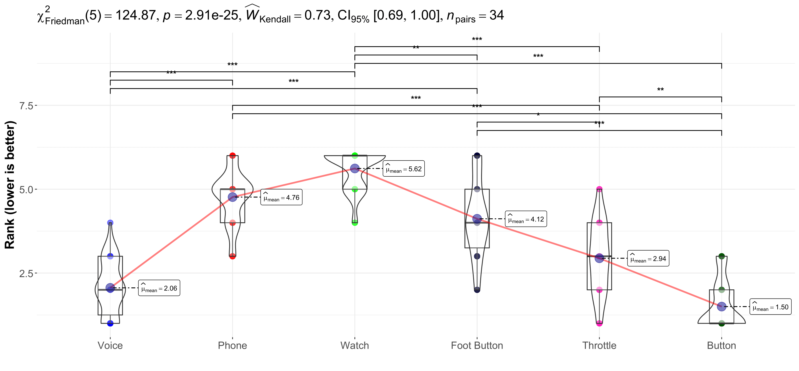
and plot_between_stats_asteriskThese functions include APA-compliant asterisks (e.g., *** for p < 0.001) on your ggwithinstats or ggbetweenstats plots. They automatically adjust for the appropriate test based on the data’s normality.
Note: Avoid using these functions if your data has more than two groups, as geom_signif does not support more than two groups.
plot_effectGenerates a plot that emphasizes either main effects or interaction effects, with clear formatting and options for publication-ready visuals. This function supports customizing group colors, axis labels, and plot size.
Example:
plot_effect(df = main_df, x = "factor1", y = "dependent_var", fillColourGroup = "group", ytext = "Y Label", xtext = "X Label", legendPos = c(0.1, 0.2), shownEffect = "interaction")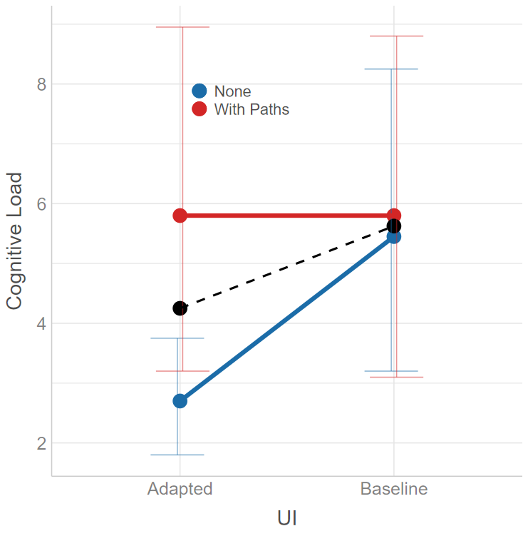
reportNPAVGenerates APA-compliant LaTeX output for within-subject designs analyzed using np.anova. The function handles both main and interaction effects. The necessary LaTeX commands are:
\newcommand{\F}[3]{$F({#1},{#2})={#3}$}
\newcommand{\p}{\textit{p=}}
\newcommand{\pminor}{\textit{p$<$}}
Deprecated: reportNPAV() is deprecated
and will be removed in a future release. Use report_art()
with ARTool instead.
Example:
model <- np.anova(tlx_mental ~ factor1 * factor2 + Error(Subject / factor1), data = main_df)
reportNPAV(model, "Dependent Variable")report_nparldReports the model produced by nparLD in APA-compliant format. For
factorial non-parametric designs, the Aligned Rank Transform
(report_art() with ARTool) is usually the more general
choice.
report_mean_sdFor each level of an independent variable, this function calculates the mean and standard deviation of a dependent variable and returns them in APA-compliant LaTeX format:
\newcommand{\m}{\textit{M=}}
\newcommand{\sd}{\textit{SD=}}
Example:
report_mean_sd(main_df, iv = "factor1", dv = "dependent_var")report_dunn_test
and report_dunn_test_tableThis function summarizes the results of FSA::dunnTest objects in text or table form. Both versions output LaTeX-ready results:
\newcommand{\padjminor}{\textit{p$_{adj}<$}}
\newcommand{\padj}{\textit{p$_{adj}$=}}
Example:
d <- dunnTest(dependent_var ~ factor1, data = main_df, method = "holm")
report_dunn_test(main_df, d, iv = "factor1", dv = "dependent_var")report_artGenerates LaTeX-formatted results from art models for factorial designs. The necessary LaTeX commands are:
\newcommand{\F}[3]{$F({#1},{#2})={#3}$}
\newcommand{\p}{\textit{p=}}
\newcommand{\pminor}{\textit{p$<$}}
Example:
model <- art(formula = dependent_var ~ factor1 * factor2 + Error(Subject / (factor1 * factor2)), data = main_df)
report_art(anova(model), "Dependent Variable")
Follow up significant effects with report_art_con() /
report_art_con_table(), which report the pairwise
art.con() contrasts as sentences or a LaTeX table
(including rank-biserial effect sizes).
add_pareto_emoa_columnThis function adds a Pareto front classification column to a dataset,
useful in multi-objective optimization scenarios.
add_pareto_moocore_column() is the equivalent based on the
moocore package (adds a PARETO_MOOCORE
column).
Attention: must be done per User - Condition etc group.
Example:
# This would do it over **all** participants and **all** conditions
objectives <- c("objective1", "objective2", "objective3")
main_df <- add_pareto_emoa_column(main_df, objectives)

# This would do it **per** participant and **per** condition combination
# (so far, does not natively support piping ``|>'')
main_df <- main_df |>
  group_by(User_ID, ConditionID) |>
  mutate(PARETO_EMOA = add_pareto_emoa_column(pick(everything()), objectives = objectives)$PARETO_EMOA) |>
  ungroup()
plot_mobo and
plot_mobo2Creates a multi-objective optimization plot, visualizing sampling and
optimization phases. This is particularly useful for visualizing
iterations in optimization problems. plot_mobo2 is
appropriate when using
https://github.com/Pascal-Jansen/Bayesian-Optimization-for-Unity/releases
starting version 1.1.0.
Example:
plot_mobo2(data = main_df, x = "Iteration", y = "objective1", fillColourGroup = "group", ytext = "Y Axis Label")Example Plot: 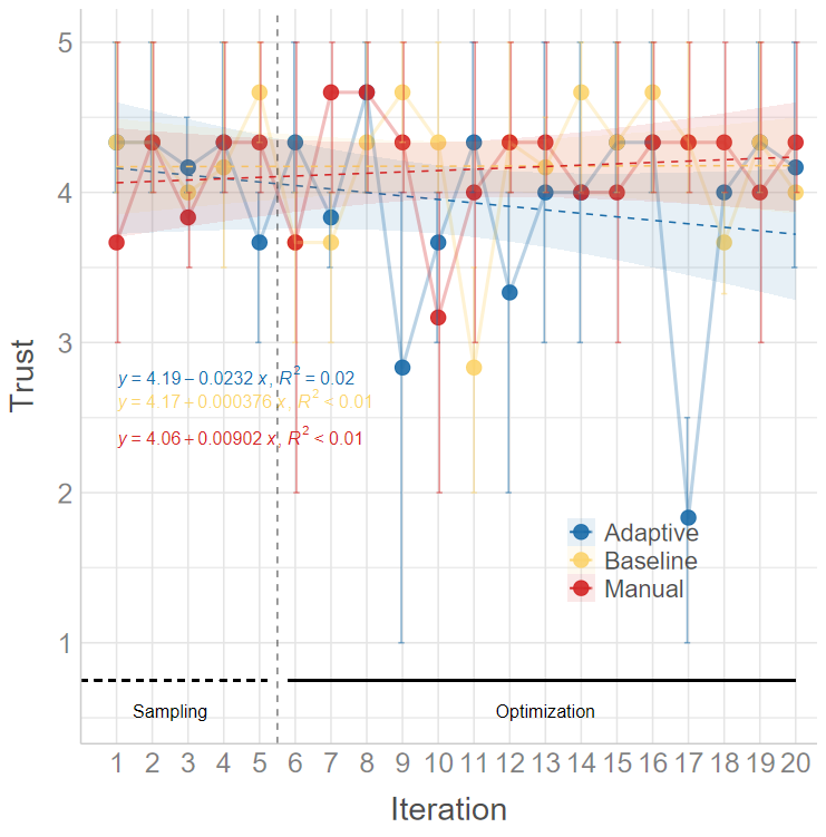
animate_mobo2Writes the same plot as a video, one frame per iteration, so a talk
or a supplement can show the run building up instead of only its end
state. The axes, phase guides and legend are taken from the complete
data, so only the points, intervals and fitted line move. Requires the
av package; the file extension picks the container
(.mp4, .gif, …).
Example:
animate_mobo2(main_df, x = "Iteration", y = "objective1", filename = "mobo.mp4", ytext = "Y Axis Label")remove_outliers_REICalculates the Response Entropy Index (REI) and flags suspicious entries based on their REI percentile. This function is useful for identifying outliers in Likert scale data.
Example:
result <- remove_outliers_REI(main_df, header = TRUE, variables = "var1,var2,var3", range = c(1, 5))replace_valuesReplaces specified values in a data frame with custom replacements. This can be used to clean or preprocess your data.
Example:
new_df <- replace_values(main_df, to_replace = c("bad_val1", "bad_val2"), replace_with = c("good_val1", "good_val2"))reportNPAV() formats results from Lüpsen’s nonparametric
ANOVA (np.anova) output. Deprecated:
reportNPAV() is deprecated and will be removed in a future
release; use report_art() with ARTool instead. NPAV is not
shipped with this package, and it is loaded manually by the user from
Lüpsen’s site: https://www.uni-koeln.de/~luepsen/R/.
This step requires internet access, so it is documented here (not in
@examples, which should run offline during package
checks).
# Download Lüpsen's NPAV bundle (anova.lib) and load it into a dedicated environment
npav_file <- tempfile(fileext = ".lib")
utils::download.file(
  url      = "https://www.uni-koeln.de/~luepsen/R/anova.lib",
  destfile = npav_file,
  mode     = "wb",
  quiet    = TRUE
)

npav_env <- new.env(parent = base::emptyenv())
base::load(npav_file, envir = npav_env)

# Example
set.seed(1)
main_df <- data.frame(
  UserID     = factor(rep(1:12, each = 8)),
  Video      = factor(rep(c("V1", "V2"), times = 48)),
  gesture    = factor(rep(c("g1", "g2"), each = 4, times = 12)),
  eHMI       = factor(rep(c("off", "on"), each = 2, times = 24)),
  tlx_mental = rnorm(96)
)

model <- npav_env$np.anova(
  tlx_mental ~ Video * gesture * eHMI + Error(UserID / (gesture * eHMI)),
  data = main_df
)

reportNPAV(model, dv = "mental workload")
If download.file() is blocked in your environment, download anova.lib manually from the NPAV page and point npav_file to the local path
For questions or remarks, please contact Mark Colley.
@misc{colley2025rstats,
  author       = {Mark Colley},
  title        = {colleyRstats: Functions to Streamline Statistical Analysis and Reporting},
  year         = {2025},
  howpublished = {\url{https://github.com/M-Colley/colleyRstats}},
  note         = {A collection of custom R functions for streamlining statistical analysis, visualizations, and APA-compliant reporting.},
  doi          = {10.5281/zenodo.18046754},
  url          = {https://doi.org/10.5281/zenodo.18046754},
}I am happy to receive any bug reports, suggestions, questions, and
contributions to fix problems and add features. Please use the
GitHub issues system. Pull Requests for contributions are
encouraged.
The following presents some simple ways in which you can contribute (in increasing order of commitment):