![]()
Dynamic Failure Rate Distributions for Survival Analysis
Capacitors that wear out faster than any Weibull can describe.
Software systems with bathtub-shaped crash rates. Post-surgical patients
whose risk drops sharply, then slowly climbs again. Standard parametric
survival families cannot express these hazard patterns — but
flexhaz can.
Write the hazard function you need — any R function of time and parameters — and the package derives everything else: survival curves, CDFs, densities, quantiles, sampling, log-likelihoods, MLE fitting, and residual diagnostics.
| Feature | flexhaz | survival | flexsurv |
|---|---|---|---|
| Custom hazard functions | Yes | No | Limited |
| Built-in distributions | Exp, Weibull, Gompertz, Log-logistic | Weibull, Exp | Many |
| User-supplied derivatives | score + Hessian | No | No |
| Censoring support | Right + Left | Right | Right |
| Model diagnostics | Cox-Snell, Martingale, Q-Q | Limited | Limited |
| Likelihood model interface | Full | Basic | Partial |
algebraic.dist, likelihood.model,
algebraic.mleInstall from CRAN:
install.packages("flexhaz")Or the development version from r-universe:
install.packages("flexhaz", repos = "https://queelius.r-universe.dev")library(flexhaz)Use the convenient constructors for classic survival distributions:
# Exponential: constant hazard (memoryless)
exp_dist <- dfr_exponential(lambda = 0.5)

# Weibull: power-law hazard (wear-out or infant mortality)
weib_dist <- dfr_weibull(shape = 2, scale = 3)

# Gompertz: exponentially increasing hazard (aging)
gomp_dist <- dfr_gompertz(a = 0.01, b = 0.1)

# Log-logistic: non-monotonic hazard (increases then decreases)
ll_dist <- dfr_loglogistic(alpha = 10, beta = 2)
All distribution functions are automatically available:
S <- surv(exp_dist)
S(2)  # Survival probability at t=2
#> [1] 0.3678794

h <- hazard(weib_dist)
h(1)  # Hazard at t=1
#> [1] 0.2222222# Simulate failure times
set.seed(42)
times <- rexp(50, rate = 1)
df <- data.frame(t = times, delta = 1)
# Fit via MLE
solver <- fit(dfr_exponential())
result <- solver(df, par = c(0.5), method = "BFGS")
coef(result) # Estimated rate
#> [1] 0.8808457Model complex failure patterns like bathtub curves:
# h(t) = a*exp(-b*t) + c + d*t^k
# Infant mortality + useful life + wear-out
bathtub <- dfr_dist(
  rate = function(t, par, ...) {
    par[1] * exp(-par[2] * t) + par[3] + par[4] * t^par[5]
  },
  par = c(a = 1, b = 2, c = 0.02, d = 0.001, k = 2)
)

h <- hazard(bathtub)
curve(sapply(x, h), 0, 15, xlab = "Time", ylab = "Hazard rate",
      main = "Bathtub hazard curve")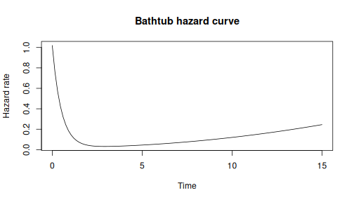
Check model fit with residual analysis:
# Fit exponential to data
fitted_exp <- dfr_exponential(lambda = coef(result))

# Cox-Snell residuals Q-Q plot
qqplot_residuals(fitted_exp, df)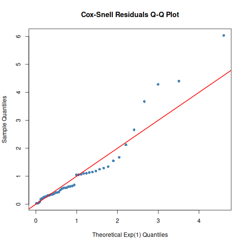
For a lifetime , the hazard function is:
From the hazard, all other quantities follow:
| Function | Formula | Method |
|---|---|---|
| Cumulative hazard | cum_haz() |
|
| Survival | surv() |
|
| CDF | cdf() |
|
density() |
For exact observations:
For right-censored:
# Mixed data with censoring
df <- data.frame(
  t = c(1, 2, 3, 4, 5),
  delta = c(1, 1, 0, 1, 0)  # 1 = exact, 0 = censored
)

ll <- loglik(dfr_exponential())
ll(df, par = c(0.5))
#> [1] -9.579442Start Here:
Real-World Applications:
Going Deeper:
Reference:
algebraic.dist:
Generic distribution interfacelikelihood.model:
Likelihood model frameworkalgebraic.mle:
MLE utilities