![]()
🌟 If you find ggpicrust2 helpful, please
consider giving us a star on GitHub! Your support greatly
motivates us to improve and maintain this project. 🌟
ggpicrust2 is a comprehensive package designed to provide a seamless and intuitive solution for analyzing and interpreting the results of PICRUSt2 functional prediction. It offers a wide range of features, including pathway name/description annotations, advanced differential abundance (DA) methods, and visualization of DA results.
One of the newest additions to ggpicrust2 is the capability to compare the consistency and inconsistency across different DA methods applied to the same dataset. This feature allows users to assess the agreement and discrepancy between various methods when it comes to predicting and sequencing the metagenome of a particular sample. It provides valuable insights into the consistency of results obtained from different approaches and helps users evaluate the robustness of their findings.
By leveraging this functionality, researchers, data scientists, and bioinformaticians can gain a deeper understanding of the underlying biological processes and mechanisms present in their PICRUSt2 output data. This comparison of different methods enables them to make informed decisions and draw reliable conclusions based on the consistency evaluation of macrogenomic predictions or sequencing results for the same sample.
If you are interested in exploring and analyzing your PICRUSt2 output data, ggpicrust2 is a powerful tool that provides a comprehensive set of features, including the ability to assess the consistency and evaluate the performance of different methods applied to the same dataset.
![]()
🔬 Enhanced GSEA with Limma Camera/Fry Methods (v2.5.6)
We’ve significantly enhanced the pathway_gsea() function
with limma’s competitive gene set testing methods:
camera method (new default): Accounts
for inter-gene correlations, providing more reliable p-values than
preranked methods (Wu et al., 2012)fry method: Fast rotation gene set
test, efficient for large gene set collectionsThis addresses concerns in the literature that preranked GSEA methods can produce “spectacularly wrong p-values” due to not accounting for inter-gene correlations.
📊 New Visualization Functions: Volcano Plot & Ridge Plot
We’ve added two new visualization functions for enhanced analysis and interpretation:
pathway_volcano(): Creates
publication-quality volcano plots for differential abundance analysis,
with smart label placement and color-coded significance categories.pathway_ridgeplot(): Creates ridge
plots (joy plots) for GSEA results interpretation, showing distribution
of gene abundances within enriched pathways.🔄 Updated Reference Databases for Improved Pathway Annotation (v2.1.4)
We’ve significantly enhanced the reference databases used for pathway annotation:
These updates provide more comprehensive and accurate pathway annotations, especially for recently discovered enzymes and KEGG orthology entries. Users will experience improved coverage and precision in pathway analysis without needing to change any code.
🌟 New Feature: Gene Set Enrichment Analysis (GSEA) for PICRUSt2 Data
We’re excited to announce the addition of GSEA functionality to the ggpicrust2 package! This powerful new feature allows researchers to perform Gene Set Enrichment Analysis on PICRUSt2 predicted functional profiles, offering a more nuanced understanding of functional differences between conditions.
The new GSEA module includes:
pathway_gsea(): Performs GSEA analysis on PICRUSt2
datavisualize_gsea(): Creates various visualizations
including enrichment plots, dot plots, network plots, and heatmapscompare_gsea_daa(): Compares GSEA and differential
abundance analysis resultsgsea_pathway_annotation(): Annotates GSEA results with
pathway informationThese new functions complement our existing differential abundance analysis tools, providing researchers with multiple approaches to analyze functional profiles.
🧫 New Feature: Taxa Contribution Workflow for PICRUSt2 Per-sequence Outputs
ggpicrust2 now supports parsing and visualizing PICRUSt2 per-sequence contribution outputs:
read_contrib_file(): Reads
pred_metagenome_contrib.tsvread_strat_file(): Reads
pred_metagenome_strat.tsvaggregate_taxa_contributions(): Aggregates
contributions by taxon, sample, and functiontaxa_contribution_bar(): Creates stacked bar plots of
taxon-level contributionstaxa_contribution_heatmap(): Summarizes contribution
patterns across taxa and functionsThis workflow makes it possible to move from pathway-level significance to an interpretable answer for which taxa are driving those pathway shifts.
🌟 Also Check Out: mLLMCelltype
We’re excited to introduce mLLMCelltype, our innovative
framework for single-cell RNA sequencing data
annotation. This iterative multi-LLM consensus framework
leverages the collective intelligence of multiple large language models
(including GPT-4o/4.1, Claude-3.7/3.5, Gemini-2.0, Grok-3, and others)
to significantly improve cell type annotation accuracy while providing
transparent uncertainty quantification.
mLLMCelltype addresses critical challenges in scRNA-seq
analysis through its unique architecture:
For researchers working with single-cell data,
mLLMCelltype offers a powerful new approach to cell type
annotation. Learn more about its capabilities and methodology on GitHub:
mLLMCelltype
Repository.
We appreciate your support and interest in our tools and look forward to seeing how they can enhance your research.
If you use ggpicrust2 in your research, please cite the following paper:
Chen Yang and others. (2023). ggpicrust2: an R package for PICRUSt2 predicted functional profile analysis and visualization. Bioinformatics, btad470. DOI link
The package citation is also available directly in R:
citation("ggpicrust2")You can install the development version of ggpicrust2 from GitHub with:
# install.packages("devtools")
devtools::install_github("cafferychen777/ggpicrust2")| Package | Description |
|---|---|
| aplot | Create interactive plots |
| dplyr | A fast consistent tool for working with data frame like objects both in memory and out of memory |
| ggplot2 | An implementation of the Grammar of Graphics in R |
| grid | A rewrite of the graphics layout capabilities of R |
| MicrobiomeStat | Statistical analysis of microbiome data |
| readr | Read rectangular data (csv tsv fwf) into R |
| stats | The R Stats Package |
| tibble | Simple Data Frames |
| tidyr | Easily tidy data with spread() and gather() functions |
| ggprism | Interactive 3D plots with ‘prism’ graphics |
| cowplot | Streamlined Plot Theme and Plot Annotations for ‘ggplot2’ |
| ggforce | Easily add secondary axes, zooms, and image overlays to ‘ggplot2’ |
| ggplotify | Convert complex plots into ‘grob’ or ‘ggplot’ objects |
| magrittr | A Forward-Pipe Operator for R |
| utils | The R Utils Package |
The package works with a minimal CRAN installation, but several workflows rely on Bioconductor packages that should be installed only when you use the corresponding analysis methods or visualizations.
| Package | Description |
|---|---|
| phyloseq | Handling and analysis of high-throughput microbiome census data |
| ALDEx2 | Differential abundance analysis of taxonomic and functional features |
| SummarizedExperiment | SummarizedExperiment container for storing data and metadata together |
| Biobase | Base functions for Bioconductor |
| devtools | Tools to make developing R packages easier |
| ComplexHeatmap | Making Complex Heatmaps in R |
| BiocGenerics | S4 generic functions for Bioconductor |
| BiocManager | Access the Bioconductor Project Package Repositories |
| metagenomeSeq | Statistical analysis for sparse high-throughput sequencing |
| Maaslin2 | Tools for microbiome analysis |
| edgeR | Empirical Analysis of Digital Gene Expression Data in R |
| lefser | R implementation of the LEfSE method for microbiome biomarker discovery |
| limma | Linear Models for Microarray and RNA-Seq Data |
| KEGGREST | R Interface to KEGG REST API |
| DESeq2 | Differential gene expression analysis using RNA-seq data |
if (!requireNamespace("BiocManager", quietly = TRUE))
    install.packages("BiocManager")

pkgs <- c("phyloseq", "ALDEx2", "SummarizedExperiment", "Biobase", "devtools",
          "ComplexHeatmap", "BiocGenerics", "BiocManager", "metagenomeSeq",
          "Maaslin2", "edgeR", "lefser", "limma", "KEGGREST", "DESeq2")

for (pkg in pkgs) {
  if (!requireNamespace(pkg, quietly = TRUE))
    BiocManager::install(pkg)
}Use the project resources below for stable updates and support:
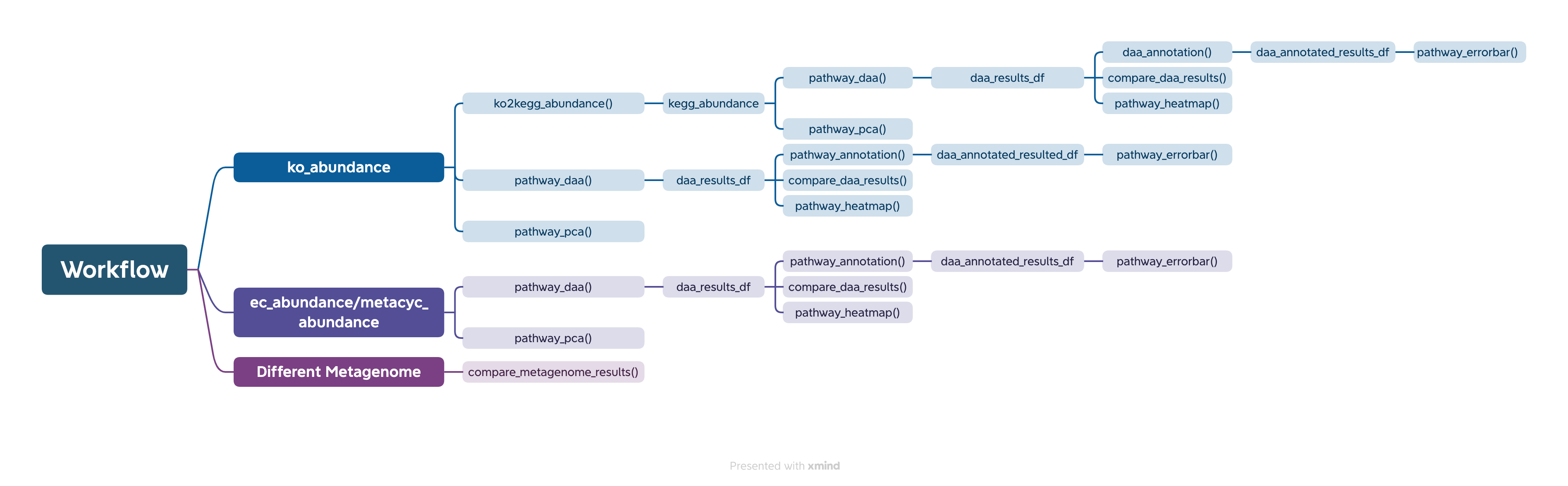
The easiest way to analyze the PICRUSt2 output is using ggpicrust2() function. The main pipeline can be run with ggpicrust2() function.
ggpicrust2() integrates ko abundance to kegg pathway abundance conversion, annotation of pathway, differential abundance (DA) analysis, part of DA results visualization. When you have trouble running ggpicrust2(), you can debug it by running a separate function, which will greatly increase the speed of your analysis and visualization.
You can download the example dataset from the provided Github link and Google Drive link or use the dataset included in the package.
# If you want to analyze the abundance of KEGG pathways instead of KO within the pathway, please set `ko_to_kegg` to TRUE.
# KEGG pathways typically have more descriptive explanations.

library(readr)
library(ggpicrust2)
library(tibble)
library(tidyverse)
library(ggprism)
library(patchwork)

# Load necessary data: abundance data and metadata
abundance_file <- "path/to/your/abundance_file.tsv"
metadata <- read_delim(
    "path/to/your/metadata.txt",
    delim = "\t",
    escape_double = FALSE,
    trim_ws = TRUE
)

# Run ggpicrust2 with input file path
results_file_input <- ggpicrust2(file = abundance_file,
                                 metadata = metadata,
                                 group = "your_group_column", # For example dataset, group = "Environment"
                                 pathway = "KO",
                                 daa_method = "LinDA",
                                 ko_to_kegg = TRUE,
                                 order = "pathway_class",
                                 p_values_bar = TRUE,
                                 x_lab = "pathway_name")

# Run ggpicrust2 with imported data.frame
abundance_data <- read_delim(abundance_file, delim = "\t", col_names = TRUE, trim_ws = TRUE)

# Run ggpicrust2 with input data
results_data_input <- ggpicrust2(data = abundance_data,
                                 metadata = metadata,
                                 group = "your_group_column", # For example dataset, group = "Environment"
                                 pathway = "KO",
                                 daa_method = "LinDA",
                                 ko_to_kegg = TRUE,
                                 order = "pathway_class",
                                 p_values_bar = TRUE,
                                 x_lab = "pathway_name")

# Access the plot and results dataframe for the first DA method
example_plot <- results_file_input[[1]]$plot
example_results <- results_file_input[[1]]$results

# Use the example data in ggpicrust2 package
data(ko_abundance)
data(metadata)
results_file_input <- ggpicrust2(data = ko_abundance,
                                 metadata = metadata,
                                 group = "Environment",
                                 pathway = "KO",
                                 daa_method = "LinDA",
                                 ko_to_kegg = TRUE,
                                 order = "pathway_class",
                                 p_values_bar = TRUE,
                                 x_lab = "pathway_name")

# Analyze the EC or MetaCyc pathway
data(metacyc_abundance)
results_file_input <- ggpicrust2(data = metacyc_abundance,
                                 metadata = metadata,
                                 group = "Environment",
                                 pathway = "MetaCyc",
                                 daa_method = "LinDA",
                                 ko_to_kegg = FALSE,
                                 order = "group",
                                 p_values_bar = TRUE,
                                 x_lab = "description")
results_file_input[[1]]$plot
results_file_input[[1]]$resultslibrary(readr)
library(ggpicrust2)
library(tibble)
library(tidyverse)
library(ggprism)
library(patchwork)
# If you want to analyze KEGG pathway abundance instead of KO within the pathway, turn ko_to_kegg to TRUE.
# KEGG pathways typically have more explainable descriptions.
# Load metadata as a tibble
# data(metadata)
metadata <- read_delim("path/to/your/metadata.txt", delim = "\t", escape_double = FALSE, trim_ws = TRUE)
# Load KEGG pathway abundance
# data(kegg_abundance)
kegg_abundance <- ko2kegg_abundance("path/to/your/pred_metagenome_unstrat.tsv")
# Perform pathway differential abundance analysis (DAA) using ALDEx2 method.
# Please change group to "your_group_column" if you are not using example dataset.
# From v2.5.14 ALDEx2 results include effect_size, diff_btw, log2_fold_change,
# rab_all, and overlap columns by default (via ALDEx2::aldex.effect()), matching
# the other DAA methods that return log2 fold changes by default. Pass
# include_effect_size = FALSE to skip that step.
daa_results_df <- pathway_daa(abundance = kegg_abundance, metadata = metadata, group = "Environment", daa_method = "ALDEx2", select = NULL, reference = NULL)
# Filter results for ALDEx2_Wilcoxon rank test method
# Please check the unique(daa_results_df$method) and choose one
daa_sub_method_results_df <- daa_results_df[daa_results_df$method == "ALDEx2_Wilcoxon rank test", ]
# Ranking by |log2_fold_change| is generally more biologically informative than
# ranking by p-value, especially for large datasets where small effects can
# reach statistical significance without being biologically meaningful.
top_hits <- daa_sub_method_results_df[order(-abs(daa_sub_method_results_df$log2_fold_change)), ]
# Annotate pathway results using KO to KEGG conversion
daa_annotated_sub_method_results_df <- pathway_annotation(pathway = "KO", daa_results_df = daa_sub_method_results_df, ko_to_kegg = TRUE)
# Generate pathway error bar plot
# Please change Group to metadata$your_group_column if you are not using example dataset
p <- pathway_errorbar(abundance = kegg_abundance, daa_results_df = daa_annotated_sub_method_results_df, Group = metadata$Environment, p_values_threshold = 0.05, order = "pathway_class", select = NULL, ko_to_kegg = TRUE, p_value_bar = TRUE, colors = NULL, x_lab = "pathway_name")
# If you want to analyze EC, MetaCyc, and KO without conversions, turn ko_to_kegg to FALSE.
# Load metadata as a tibble
# data(metadata)
metadata <- read_delim("path/to/your/metadata.txt", delim = "\t", escape_double = FALSE, trim_ws = TRUE)
# Load KO abundance as a data.frame
# data(ko_abundance)
ko_abundance <- read.delim("path/to/your/pred_metagenome_unstrat.tsv")
# Perform pathway DAA using ALDEx2 method
# Please change column_to_rownames() to the feature column if you are not using example dataset
# Please change group to "your_group_column" if you are not using example dataset
# ALDEx2 effect size columns (effect_size, diff_btw, log2_fold_change, rab_all,
# overlap) are included by default; see the section above.
daa_results_df <- pathway_daa(abundance = ko_abundance %>% column_to_rownames("#NAME"), metadata = metadata, group = "Environment", daa_method = "ALDEx2", select = NULL, reference = NULL)
# Filter results for ALDEx2_Wilcoxon rank test method
daa_sub_method_results_df <- daa_results_df[daa_results_df$method == "ALDEx2_Wilcoxon rank test", ]
# Annotate pathway results without KO to KEGG conversion
daa_annotated_sub_method_results_df <- pathway_annotation(pathway = "KO", daa_results_df = daa_sub_method_results_df, ko_to_kegg = FALSE)
# Generate pathway error bar plot
# Please change column_to_rownames() to the feature column
# Please change Group to metadata$your_group_column if you are not using example dataset
p <- pathway_errorbar(abundance = ko_abundance %>% column_to_rownames("#NAME"), daa_results_df = daa_annotated_sub_method_results_df, Group = metadata$Environment, p_values_threshold = 0.05, order = "group",
select = daa_annotated_sub_method_results_df %>% arrange(p_adjust) %>% slice(1:20) %>% dplyr::select(feature) %>% pull(),
ko_to_kegg = FALSE,
p_value_bar = TRUE,
colors = NULL,
x_lab = "description")
# Workflow for MetaCyc Pathway and EC
# Load MetaCyc pathway abundance and metadata
data("metacyc_abundance")
data("metadata")
# Perform pathway DAA using LinDA method
# Please change column_to_rownames() to the feature column if you are not using example dataset
# Please change group to "your_group_column" if you are not using example dataset
metacyc_daa_results_df <- pathway_daa(abundance = metacyc_abundance %>% column_to_rownames("pathway"), metadata = metadata, group = "Environment", daa_method = "LinDA")
# Annotate MetaCyc pathway results without KO to KEGG conversion
metacyc_daa_annotated_results_df <- pathway_annotation(pathway = "MetaCyc", daa_results_df = metacyc_daa_results_df, ko_to_kegg = FALSE)
# Generate pathway error bar plot
# Please change column_to_rownames() to the feature column
# Please change Group to metadata$your_group_column if you are not using example dataset
pathway_errorbar(abundance = metacyc_abundance %>% column_to_rownames("pathway"), daa_results_df = metacyc_daa_annotated_results_df, Group = metadata$Environment, ko_to_kegg = FALSE, p_values_threshold = 0.05, order = "group", select = NULL, p_value_bar = TRUE, colors = NULL, x_lab = "description")
# Generate pathway heatmap
# Please change column_to_rownames() to the feature column if you are not using example dataset
# Please change group to "your_group_column" if you are not using example dataset
feature_with_p_0.05 <- metacyc_daa_results_df %>% filter(p_adjust < 0.05)
pathway_heatmap(abundance = metacyc_abundance %>% filter(pathway %in% feature_with_p_0.05$feature) %>% column_to_rownames("pathway"), metadata = metadata, group = "Environment")
# Generate pathway PCA plot
# Please change column_to_rownames() to the feature column if you are not using example dataset
# Please change group to "your_group_column" if you are not using example dataset
pathway_pca(abundance = metacyc_abundance %>% column_to_rownames("pathway"), metadata = metadata, group = "Environment")
# Run pathway DAA for multiple methods
# Please change column_to_rownames() to the feature column if you are not using example dataset
# Please change group to "your_group_column" if you are not using example dataset
methods <- c("ALDEx2", "DESeq2", "edgeR")
daa_results_list <- lapply(methods, function(method) {
pathway_daa(abundance = metacyc_abundance %>% column_to_rownames("pathway"), metadata = metadata, group = "Environment", daa_method = method)
})
# Compare results across different methods
comparison_results <- compare_daa_results(daa_results_list = daa_results_list, method_names = c("ALDEx2_Welch's t test", "ALDEx2_Wilcoxon rank test", "DESeq2", "edgeR"))The typical output of the ggpicrust2 is like this.
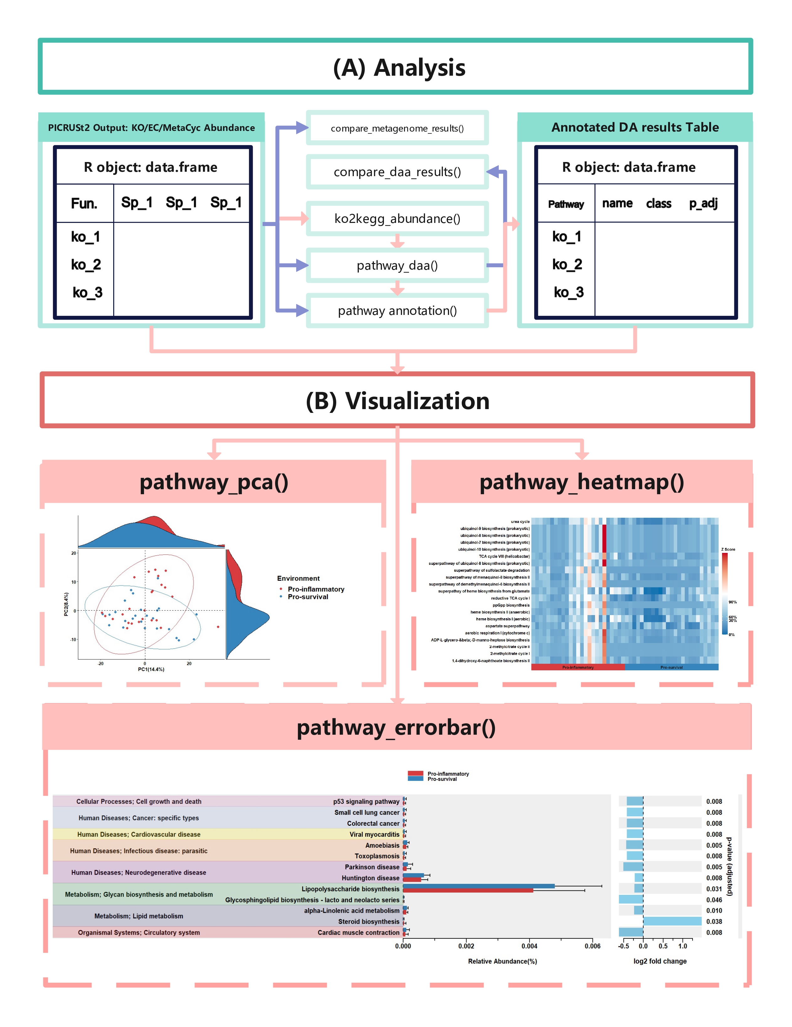
KEGG Orthology(KO) is a classification system developed by the Kyoto Encyclopedia of Genes and Genomes (KEGG) data-base(Kanehisa et al., 2022). It uses a hierarchical structure to classify enzymes based on the reactions they catalyze. To better understand pathways’ role in different groups and classify the pathways, the KO abundance table needs to be converted to KEGG pathway abundance. But PICRUSt2 removes the function from PICRUSt. ko2kegg_abundance() can help convert the table.
# Sample usage of the ko2kegg_abundance function
devtools::install_github('cafferychen777/ggpicrust2')

library(ggpicrust2)

# Assume that the KO abundance table is stored in a file named "ko_abundance.tsv"
ko_abundance_file <- "ko_abundance.tsv"

# Convert KO abundance to KEGG pathway abundance
kegg_abundance <- ko2kegg_abundance(file = ko_abundance_file)

# Alternatively, if the KO abundance data is already loaded as a data frame named "ko_abundance"
data("ko_abundance")
kegg_abundance <- ko2kegg_abundance(data = ko_abundance)

# The resulting kegg_abundance data frame can now be used for further analysis and visualization.Differential abundance (DA) analysis plays a major role in PICRUSt2
downstream analysis. pathway_daa() integrates the main DA
methods used for predicted functional profiles, excluding ANCOM and
ANCOMBC. It includes ALDEx2
(Fernandes et al., 2013), DESeq2
(Love et al., 2014), Maaslin2
(Mallick et al., 2021), LinDA (Zhou et
al., 2022), edgeR
(Robinson et al., 2010), limma
voom (Ritchie et al., 2015), metagenomeSeq
(Paulson et al., 2013), and Lefser
(Segata et al., 2011).
# The abundance table is recommended to be a data.frame rather than a tibble.
# The abundance table should have feature names or pathway names as row names, and sample names as column names.
# You can use the output of ko2kegg_abundance
ko_abundance_file <- "path/to/your/pred_metagenome_unstrat.tsv"
kegg_abundance <- ko2kegg_abundance(ko_abundance_file) # Or use data(kegg_abundance)

metadata <- read_delim("path/to/your/metadata.txt", delim = "\t", escape_double = FALSE, trim_ws = TRUE)

# The default DAA method is "ALDEx2"
# Please change group to "your_group_column" if you are not using example dataset
daa_results_df <- pathway_daa(abundance = kegg_abundance, metadata = metadata, group = "Environment", daa_method = "LinDA", select = NULL, p_adjust_method = "BH", reference = NULL)

# If you have more than 3 group levels and want to use the LinDA, limma voom, or Maaslin2 methods, you should provide a reference.
metadata <- read_delim("path/to/your/metadata.txt", delim = "\t", escape_double = FALSE, trim_ws = TRUE)

# Please change group to "your_group_column" if you are not using example dataset
daa_results_df <- pathway_daa(abundance = kegg_abundance, metadata = metadata, group = "Group", daa_method = "LinDA", select = NULL, p_adjust_method = "BH", reference = "Harvard BRI")

# Other example
data("metacyc_abundance")
data("metadata")
metacyc_daa_results_df <- pathway_daa(abundance = metacyc_abundance %>% column_to_rownames("pathway"), metadata = metadata, group = "Environment", daa_method = "LinDA", select = NULL, p_adjust_method = "BH", reference = NULL)library(ggpicrust2)
library(tidyverse)
data("metacyc_abundance")
data("metadata")
# Run pathway_daa function for multiple methods
# Please change column_to_rownames() to the feature column if you are not using example dataset
# Please change group to "your_group_column" if you are not using example dataset
methods <- c("ALDEx2", "DESeq2", "edgeR")
daa_results_list <- lapply(methods, function(method) {
pathway_daa(abundance = metacyc_abundance %>% column_to_rownames("pathway"), metadata = metadata, group = "Environment", daa_method = method)
})
method_names <- c("ALDEx2","DESeq2", "edgeR")
# Compare results across different methods
comparison_results <- compare_daa_results(daa_results_list = daa_results_list, method_names = method_names)If you are in China and you are using kegg pathway annotation, Please make sure your internet can break through the firewall.
New Feature (v2.1.4): The
pathway_annotation() function now supports species-specific
KEGG pathway annotation through the new organism parameter.
You can specify KEGG organism codes (e.g., “hsa” for human, “eco” for E.
coli) to get species-specific pathway information. If no organism is
specified (default), the function retrieves generic KO information not
specific to any organism.
Note: When ko_to_kegg = TRUE, only
pathways with p_adjust < p_adjust_threshold are sent to
the KEGG API for annotation. The p_adjust_threshold
parameter defaults to 0.05 and can be customized. When called from
ggpicrust2(), this threshold is automatically set to match
the p_values_threshold parameter for consistency.
# Make sure to check if the features in `daa_results_df` correspond to the selected pathway

# Annotate KEGG Pathway
data("kegg_abundance")
data("metadata")
# Please change group to "your_group_column" if you are not using example dataset
daa_results_df <- pathway_daa(abundance = kegg_abundance, metadata = metadata, group = "Environment", daa_method = "LinDA")

# Generic KO to KEGG pathway annotation (not specific to any organism)
daa_annotated_results_df <- pathway_annotation(pathway = "KO", daa_results_df = daa_results_df, ko_to_kegg = TRUE)

# Species-specific KEGG pathway annotation (e.g., for human)
human_annotated_results_df <- pathway_annotation(pathway = "KO", daa_results_df = daa_results_df, ko_to_kegg = TRUE, organism = "hsa")

# Species-specific KEGG pathway annotation (e.g., for E. coli)
ecoli_annotated_results_df <- pathway_annotation(pathway = "KO", daa_results_df = daa_results_df, ko_to_kegg = TRUE, organism = "eco")

# Annotate KO
data("ko_abundance")
data("metadata")
# Please change column_to_rownames() to the feature column if you are not using example dataset
# Please change group to "your_group_column" if you are not using example dataset
daa_results_df <- pathway_daa(abundance = ko_abundance %>% column_to_rownames("#NAME"), metadata = metadata, group = "Environment", daa_method = "LinDA")
daa_annotated_results_df <- pathway_annotation(pathway = "KO", daa_results_df = daa_results_df, ko_to_kegg = FALSE)

# Annotate KEGG
# daa_annotated_results_df <- pathway_annotation(pathway = "EC", daa_results_df = daa_results_df, ko_to_kegg = FALSE)

# Annotate MetaCyc Pathway
data("metacyc_abundance")
data("metadata")
# Please change column_to_rownames() to the feature column if you are not using example dataset
# Please change group to "your_group_column" if you are not using example dataset
metacyc_daa_results_df <- pathway_daa(abundance = metacyc_abundance %>% column_to_rownames("pathway"), metadata = metadata, group = "Environment", daa_method = "LinDA")
metacyc_daa_annotated_results_df <- pathway_annotation(pathway = "MetaCyc", daa_results_df = metacyc_daa_results_df, ko_to_kegg = FALSE)data("ko_abundance")
data("metadata")
kegg_abundance <- ko2kegg_abundance(data = ko_abundance) # Or use data(kegg_abundance)
# Please change group to "your_group_column" if you are not using example dataset
daa_results_df <- pathway_daa(kegg_abundance, metadata = metadata, group = "Environment", daa_method = "LinDA")
daa_annotated_results_df <- pathway_annotation(pathway = "KO", daa_results_df = daa_results_df, ko_to_kegg = TRUE)
# Please change Group to metadata$your_group_column if you are not using example dataset
p <- pathway_errorbar(abundance = kegg_abundance,
daa_results_df = daa_annotated_results_df,
Group = metadata$Environment,
ko_to_kegg = TRUE,
p_values_threshold = 0.05,
order = "pathway_class",
select = NULL,
p_value_bar = TRUE,
colors = NULL,
x_lab = "pathway_name")
# If you want to analysis the EC. MetaCyc. KO without conversions.
data("metacyc_abundance")
data("metadata")
metacyc_daa_results_df <- pathway_daa(abundance = metacyc_abundance %>% column_to_rownames("pathway"), metadata = metadata, group = "Environment", daa_method = "LinDA")
metacyc_daa_annotated_results_df <- pathway_annotation(pathway = "MetaCyc", daa_results_df = metacyc_daa_results_df, ko_to_kegg = FALSE)
p <- pathway_errorbar(abundance = metacyc_abundance %>% column_to_rownames("pathway"),
daa_results_df = metacyc_daa_annotated_results_df,
Group = metadata$Environment,
ko_to_kegg = FALSE,
p_values_threshold = 0.05,
order = "group",
select = NULL,
p_value_bar = TRUE,
colors = NULL,
x_lab = "description")In this section, we will demonstrate how to create a pathway heatmap
using the pathway_heatmap function in the ggpicrust2
package. This function visualizes the relative abundance of pathways in
different samples.
Use the fake dataset
# Create example functional pathway abundance data
abundance_example <- matrix(rnorm(30), nrow = 3, ncol = 10)
colnames(abundance_example) <- paste0("Sample", 1:10)
rownames(abundance_example) <- c("PathwayA", "PathwayB", "PathwayC")

# Create example metadata
# Please change your sample id's column name to sample_name
metadata_example <- data.frame(sample_name = colnames(abundance_example),
                               group = factor(rep(c("Control", "Treatment"), each = 5)))

# Create a heatmap
pathway_heatmap(abundance_example, metadata_example, "group")
Use the real dataset
library(tidyverse)
library(ggh4x)
library(ggpicrust2)
# Load the data
data("metacyc_abundance")

# Load the metadata
data("metadata")

# Perform differential abundance analysis
metacyc_daa_results_df <- pathway_daa(
  abundance = metacyc_abundance %>% column_to_rownames("pathway"),
  metadata = metadata,
  group = "Environment",
  daa_method = "LinDA"
)

# Annotate the results
annotated_metacyc_daa_results_df <- pathway_annotation(
  pathway = "MetaCyc",
  daa_results_df = metacyc_daa_results_df,
  ko_to_kegg = FALSE
)

# Filter features with p < 0.05
feature_with_p_0.05 <- metacyc_daa_results_df %>%
  filter(p_adjust < 0.05)

# Create the heatmap
pathway_heatmap(
  abundance = metacyc_abundance %>%
    right_join(
      annotated_metacyc_daa_results_df %>% select(all_of(c("feature","description"))),
      by = c("pathway" = "feature")
    ) %>%
    filter(pathway %in% feature_with_p_0.05$feature) %>%
    select(-"pathway") %>%
    column_to_rownames("description"),
  metadata = metadata,
  group = "Environment"
)In this section, we will demonstrate how to perform Principal
Component Analysis (PCA) on functional pathway abundance data and create
visualizations of the PCA results using the pathway_pca
function in the ggpicrust2 package.
Use the fake dataset
# Create example functional pathway abundance data
abundance_example <- matrix(rnorm(30), nrow = 3, ncol = 10)
colnames(kegg_abundance_example) <- paste0("Sample", 1:10)
rownames(kegg_abundance_example) <- c("PathwayA", "PathwayB", "PathwayC")

# Create example metadata
metadata_example <- data.frame(sample_name = colnames(kegg_abundance_example),
                                group = factor(rep(c("Control", "Treatment"), each = 5)))
# Perform PCA and create visualizations
pathway_pca(abundance = abundance_example, metadata = metadata_example, "group")
Use the real dataset
# Create example functional pathway abundance data
data("metacyc_abundance")
data("metadata")

pathway_pca(abundance = metacyc_abundance %>% column_to_rownames("pathway"), metadata = metadata, group = "Environment")library(ComplexHeatmap)
set.seed(123)
# First metagenome
metagenome1 <- abs(matrix(rnorm(1000), nrow = 100, ncol = 10))
rownames(metagenome1) <- paste0("KO", 1:100)
colnames(metagenome1) <- paste0("sample", 1:10)
# Second metagenome
metagenome2 <- abs(matrix(rnorm(1000), nrow = 100, ncol = 10))
rownames(metagenome2) <- paste0("KO", 1:100)
colnames(metagenome2) <- paste0("sample", 1:10)
# Put the metagenomes into a list
metagenomes <- list(metagenome1, metagenome2)
# Define names
names <- c("metagenome1", "metagenome2")
# Call the function
results <- compare_metagenome_results(metagenomes, names)
# Print the correlation matrix
print(results$correlation$cor_matrix)
# Print the p-value matrix
print(results$correlation$p_matrix)The taxa contribution workflow connects PICRUSt2 contribution outputs
with downstream pathway interpretation. Use
read_contrib_file() for
pred_metagenome_contrib.tsv,
read_pathway_contrib_file() for pathway-level
path_abun_contrib.tsv, or read_strat_file()
for pred_metagenome_strat.tsv, then aggregate to the
taxonomic level you want to visualize.
library(ggpicrust2)

# Parse PICRUSt2 per-sequence contribution output
contrib_data <- read_contrib_file("pred_metagenome_contrib.tsv")

# Or parse pathway-level contribution output without running DA analysis
# PICRUSt2 pathway contribution files are often gzipped and use MetaCyc IDs.
path_contrib_data <- read_pathway_contrib_file("path_abun_contrib.tsv.gz")

# Optional: use pathway-level DAA results to keep only significant pathways
data("kegg_abundance")
data("metadata")

daa_results <- pathway_daa(
  abundance = kegg_abundance,
  metadata = metadata,
  group = "Environment",
  daa_method = "ALDEx2"
)

# Aggregate contributions to genus level and keep top taxa
taxa_contrib <- aggregate_taxa_contributions(
  contrib_data = contrib_data,
  taxonomy = your_taxonomy_table,
  tax_level = "Genus",
  top_n = 10,
  daa_results_df = daa_results
)

# Visualize per-sample contributions
taxa_contribution_bar(
  contrib_agg = taxa_contrib,
  metadata = metadata,
  group = "Environment",
  facet_by = "function"
)

# Summarize mean contribution patterns across taxa and functions
taxa_contribution_heatmap(
  contrib_agg = taxa_contrib,
  n_functions = 20
)

# Pathway-level contribution workflow without DA filtering
path_taxa_contrib <- aggregate_taxa_contributions(
  contrib_data = path_contrib_data,
  taxonomy = your_taxonomy_table,
  tax_level = "Genus",
  top_n = 10
)

pathway_annotation_df <- pathway_annotation(
  data = data.frame(function_id = unique(path_taxa_contrib$function_id)),
  pathway = "MetaCyc"
)

taxa_contribution_heatmap(
  contrib_agg = path_taxa_contrib,
  annotation_data = pathway_annotation_df,
  n_functions = 20
)The pathway_gsea() function performs Gene Set Enrichment
Analysis (GSEA) on PICRUSt2 predicted functional profiles. GSEA is a
powerful method for identifying enriched pathways between different
conditions, offering a more nuanced understanding of functional
differences compared to traditional differential abundance analysis.
New in v2.5.6: The function now supports limma’s
camera and fry methods, which provide more
reliable p-values by accounting for inter-gene correlations (Wu et al.,
2012). The camera method is now the default and recommended
approach.
| Method | Type | Covariate Support | Description |
|---|---|---|---|
camera (default) |
Competitive | ✅ Yes | Recommended. Accounts for inter-gene correlations |
fry |
Self-contained | ✅ Yes | Fast rotation test, efficient for large gene set collections |
fgsea |
Preranked | ❌ No | Fast preranked GSEA (legacy) |
clusterProfiler |
Preranked | ❌ No | Traditional GSEA implementation (legacy) |
library(ggpicrust2)
library(tidyverse)

# Load example data
data("ko_abundance")
data("metadata")

# Perform GSEA analysis with camera (recommended)
gsea_results <- pathway_gsea(
  abundance = ko_abundance %>% column_to_rownames("#NAME"),
  metadata = metadata,
  group = "Environment",
  method = "camera",   # Recommended: accounts for inter-gene correlations
  pathway_type = "KEGG",
  min_size = 5,
  max_size = 500
)

# With covariate adjustment (powerful feature of camera/fry)
gsea_results_adjusted <- pathway_gsea(
  abundance = ko_abundance %>% column_to_rownames("#NAME"),
  metadata = metadata,
  group = "Disease",
  covariates = c("age", "sex"),  # Adjust for confounders
  method = "camera",
  pathway_type = "KEGG"
)

# View the results
head(gsea_results)The visualize_gsea() function creates various
visualizations for GSEA results, including enrichment plots, dot plots,
network plots, and heatmaps.
library(ggpicrust2)
library(tidyverse)

# Load example data and perform GSEA
data("ko_abundance")
data("metadata")

gsea_results <- pathway_gsea(
  abundance = ko_abundance %>% column_to_rownames("#NAME"),
  metadata = metadata,
  group = "Environment"
)

# Create an enrichment plot for a specific pathway
# Annotate results so plots can use readable pathway names
annotated_results <- gsea_pathway_annotation(
  gsea_results = gsea_results,
  pathway_type = "KEGG"
)

# Create an enrichment-style summary plot
enrichment_plot <- visualize_gsea(
  gsea_results = annotated_results,
  plot_type = "enrichment_plot",
  n_pathways = 10
)

# Create a dot plot showing top enriched pathways
dot_plot <- visualize_gsea(
  gsea_results = annotated_results,
  plot_type = "dotplot",
  n_pathways = 20,  # Show top 20 pathways
  sort_by = "NES"   # Sort by Normalized Enrichment Score
)

# Create a network plot showing pathway relationships
network_plot <- visualize_gsea(
  gsea_results = gsea_results,
  plot_type = "network",
  n_pathways = 15,
  network_params = list(
    similarity_measure = "jaccard",
    similarity_cutoff = 0.2,
    layout = "fruchterman",
    node_color_by = "NES"
  )
)

# Create a heatmap showing pathway gene expression
heatmap_plot <- visualize_gsea(
  gsea_results = gsea_results,
  plot_type = "heatmap",
  abundance = ko_abundance %>% column_to_rownames("#NAME"),
  metadata = metadata,
  group = "Environment",
  n_pathways = 10,
  heatmap_params = list(
    cluster_rows = TRUE,
    cluster_columns = TRUE,
    show_column_names = TRUE,
    show_row_names = FALSE
  )
)The compare_gsea_daa() function compares results from
GSEA and differential abundance analysis (DAA) to identify pathways that
are consistently identified by both methods or uniquely identified by
each method.
library(ggpicrust2)
library(tidyverse)

# Load example data
data("ko_abundance")
data("metadata")

# Prepare pathway-level abundance for DAA so identifiers match GSEA pathway IDs
kegg_pathway_abundance <- ko2kegg_abundance(data = ko_abundance)

# Perform GSEA analysis
gsea_results <- pathway_gsea(
  abundance = ko_abundance %>% column_to_rownames("#NAME"),
  metadata = metadata,
  group = "Environment"
)

# Perform DAA analysis
daa_results <- pathway_daa(
  abundance = kegg_pathway_abundance,
  metadata = metadata,
  group = "Environment",
  daa_method = "ALDEx2"
)

# Compare GSEA and DAA results
comparison <- compare_gsea_daa(
  gsea_results = gsea_results,
  daa_results = daa_results,
  p_threshold = 0.05,
  plot_type = "venn"  # Can be "venn", "upset", or "scatter"
)

# View the comparison plot
comparison$plot

# View the overlapping pathways
head(comparison$results$overlap)The gsea_pathway_annotation() function annotates GSEA
results with pathway information, including pathway names, descriptions,
and classifications.
library(ggpicrust2)
library(tidyverse)

# Load example data and perform GSEA
data("ko_abundance")
data("metadata")

gsea_results <- pathway_gsea(
  abundance = ko_abundance %>% column_to_rownames("#NAME"),
  metadata = metadata,
  group = "Environment"
)

# Annotate GSEA results
annotated_results <- gsea_pathway_annotation(
  gsea_results = gsea_results,
  pathway_type = "KEGG"
)

# View the annotated results
head(annotated_results)When using pathway_errorbar with the following
parameters:
pathway_errorbar(abundance = abundance,
                 daa_results_df = daa_results_df,
                 Group = metadata$Environment,
                 ko_to_kegg = TRUE,
                 p_values_threshold = 0.05,
                 order = "pathway_class",
                 select = NULL,
                 p_value_bar = TRUE,
                 colors = NULL,
                 x_lab = "pathway_name")
You may encounter an error:
Error in `ggplot_add()`:
! Can't add `e2` to a <ggplot> object.
Run `rlang::last_trace()` to see where the error occurred.
Make sure you have the patchwork package loaded:
library(patchwork)You may encounter an error with
guide_train.prism_offset_minor:
Error in guide_train.prism_offset_minor(guide, panel_params[[aesthetic]]) :
  No minor breaks exist, guide_prism_offset_minor needs minor breaks to work

Error in get(as.character(FUN),mode = "function"object envir = envir)
guide_prism_offset_minor' of mode'function' was not found
Ensure that the ggprism package is loaded:
library(ggprism)When encountering the following error:
SSL peer certificate or SSH remote key was not OK: [rest.kegg.jp] SSL certificate problem: certificate has expiredIf you are in China, make sure your computer network can bypass the firewall.
When encountering the following error:
Error in .getUrl(url, .flatFileParser) : Bad Request (HTTP 400).Please restart R session.
When encountering the following error:
Error in grid.Call(C_textBounds, as.graphicsAnnot(xlabel),x$x, x$y, :Please having some required fonts installed. You can refer to this thread.
When faced with this issue, consider the following solutions:
Solution 1: Utilize the ‘select’ parameter
The ‘select’ parameter allows you to specify which features you wish to visualize. Here’s an example of how you can apply this in your code:
ggpicrust2::pathway_errorbar(
  abundance = kegg_abundance,
  daa_results_df = daa_results_df_annotated,
  Group = metadata$Day,
  p_values_threshold = 0.05,
  order = "pathway_class",
  select = c("ko05340", "ko00564", "ko00680", "ko00562", "ko03030", "ko00561", "ko00440", "ko00250", "ko00740", "ko04940", "ko00010", "ko00195", "ko00760", "ko00920", "ko00311", "ko00310", "ko04146", "ko00600", "ko04141", "ko04142", "ko00604", "ko04260", "ko00909", "ko04973", "ko00510", "ko04974"),
  ko_to_kegg = TRUE,
  p_value_bar = FALSE,
  colors = NULL,
  x_lab = "pathway_name"
)
Solution 2: Limit to the Top 20 features
If there are too many significant features to visualize effectively, you might consider limiting your visualization to the top 20 features with the smallest adjusted p-values:
daa_results_df_annotated <- daa_results_df_annotated[!is.na(daa_results_df_annotated$pathway_name),]

daa_results_df_annotated$p_adjust <- round(daa_results_df_annotated$p_adjust,5)

low_p_feature <- daa_results_df_annotated[order(daa_results_df_annotated$p_adjust), ]$feature[1:20]


p <- ggpicrust2::pathway_errorbar(
  abundance = kegg_abundance,
  daa_results_df = daa_results_df_annotated,
  Group = metadata$Day,
  p_values_threshold = 0.05,
  order = "pathway_class",
  select = low_p_feature,
  ko_to_kegg = TRUE,
  p_value_bar = FALSE,
  colors = NULL,
x_lab = "pathway_name")If you are not finding any statistically significant biomarkers in your analysis, there could be several reasons for this:
The true difference between your groups is small or non-existent. If the microbial communities or pathways you’re comparing are truly similar, then it’s correct and expected that you won’t find significant differences.
Your sample size might be too small to detect the differences. Statistical power, the ability to detect differences if they exist, increases with sample size.
The variation within your groups might be too large. If there’s a lot of variation in microbial communities within a single group, it can be hard to detect differences between groups.
Here are a few suggestions:
Increase your sample size: If possible, adding more samples to your analysis can increase your statistical power, making it easier to detect significant differences.
Decrease intra-group variation: If there’s a lot of variation within your groups, consider whether there are outliers or subgroups that are driving this variation. You might need to clean your data, or to stratify your analysis to account for these subgroups.
Change your statistical method or adjust parameters: Depending on the nature of your data and your specific question, different statistical methods might be more or less powerful. If you’re currently using a parametric test, consider using a non-parametric test, or vice versa. Also, consider whether adjusting the parameters of your current test might help.
Remember, not finding significant results is also a result and can be informative, as it might indicate that there are no substantial differences between the groups you’re studying. It’s important to interpret your results in the context of your specific study and not to force statistical significance where there isn’t any.
With these strategies, you should be able to create a more readable and informative visualization, even when dealing with a large number of significant features.
If you’re interested in helping to test and develop MicrobiomeStat, please contact cafferychen7850@gmail.com.

We look forward to sharing more updates as these projects progress.