healthyR.ts

The Time Series Modeling Companion to healthyR

To view the full wiki, click here: Full healthyR.ts Wiki

healthyR.ts is a comprehensive R package designed specifically for time series analysis and forecasting of hospital administrative and clinical data. Built on the powerful tidymodels ecosystem, it provides a consistent, user-friendly framework that simplifies complex time series workflows.

Why healthyR.ts?

Hospital data analysis often requires handling time series for metrics like: - Average Length of Stay (ALOS) - Readmission rates - Patient volumes and admissions - Bed occupancy rates - Clinical outcomes over time

healthyR.ts takes the guesswork out of time series analysis by providing:

✅ Automated Workflows - One-function solutions for complete modeling pipelines
✅ Visual Analytics - Rich plotting functions for data exploration
✅ Data Generators - Simulate realistic time series for testing and validation
✅ Statistical Tools - Comprehensive suite of time series statistics
✅ Clustering - Feature-based time series clustering capabilities
✅ Forecasting - 15 automated model workflows (ARIMA, Prophet, XGBoost, and more)

Key Features

🤖 Automatic Modeling Workflows

Complete end-to-end modeling pipelines in a single function call:

ts_auto_arima() - Automatic ARIMA modeling
ts_auto_prophet_reg() - Facebook’s Prophet algorithm
ts_auto_xgboost() - Gradient boosting for time series
ts_auto_nnetar() - Neural network autoregression
Plus 11 more specialized workflows!

Each function handles recipe creation, model specification, workflow setup, model fitting, tuning, and calibration automatically.

📊 Visualization Suite

Calendar heatmaps for temporal patterns
Time series clustering plots
Velocity, acceleration, and growth visualizations
QQ plots and scedasticity analysis
Moving average and SMA plots
Event analysis visualizations

🎲 Data Generation

Generate synthetic time series data for testing: - Random walks and Brownian motion - Geometric Brownian motion - ARIMA simulations - Custom parameter configurations

📈 Statistical Analysis

ADF stationarity tests
Fast Fourier Transform (FFT) analysis
Confidence intervals
Lag correlation analysis
Time series feature extraction

Installation

Stable Release (CRAN)

Install the latest stable version from CRAN:

install.packages("healthyR.ts")

Development Version

Get the latest features and bug fixes from GitHub:

# install.packages("devtools")
devtools::install_github("spsanderson/healthyR.ts")

Quick Start

Basic Example: Random Walk Simulation

Generate and visualize random walk data to understand market volatility or patient flow variations:

library(healthyR.ts)
library(ggplot2)

df <- ts_random_walk()

head(df)
#> # A tibble: 6 × 4
#>     run     x       y cum_y
#>   <dbl> <dbl>   <dbl> <dbl>
#> 1     1     1  0.113  1113.
#> 2     1     2  0.119  1245.
#> 3     1     3 -0.0178 1223.
#> 4     1     4  0.141  1396.
#> 5     1     5 -0.163  1169.
#> 6     1     6 -0.0485 1112.

Now that the data has been generated, lets take a look at it.

df %>%
   ggplot(
       mapping = aes(
           x = x
           , y = cum_y
           , color = factor(run)
           , group = factor(run)
        )
    ) +
    geom_line(alpha = 0.8) +
    ts_random_walk_ggplot_layers(df)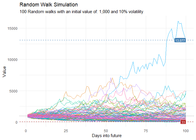

That is still pretty noisy, so lets see this in a different way. Lets clear this up a bit to make it easier to see the full range of the possible volatility of the random walks.

library(dplyr)
library(ggplot2)

df %>%
    group_by(x) %>%
    summarise(
        min_y = min(cum_y),
        max_y = max(cum_y)
    ) %>%
    ggplot(
        aes(x = x)
    ) +
    geom_line(aes(y = max_y), color = "steelblue") +
    geom_line(aes(y = min_y), color = "firebrick") +
    geom_ribbon(aes(ymin = min_y, ymax = max_y), alpha = 0.2) +
    ts_random_walk_ggplot_layers(df)

Calendar Heatmap Visualization

Visualize temporal patterns in your data with calendar heatmaps - perfect for identifying seasonal trends or unusual patterns in hospital metrics:

data_tbl <- data.frame(
  date_col = seq.Date(
    from = as.Date("2020-01-01"),
    to   = as.Date("2022-06-01"),
    length.out = 365*2 + 180
    ),
  value = rnorm(365*2+180, mean = 100)
)

ts_calendar_heatmap_plot(
  .data          = data_tbl
  , .date_col    = date_col
  , .value_col   = value
  , .interactive = FALSE
)

Time Series Clustering

Discover patterns by clustering time series based on their statistical features:

data_tbl <- ts_to_tbl(AirPassengers) %>%
  mutate(group_id = rep(1:12, 12))

output <- ts_feature_cluster(
  .data = data_tbl,
  .date_col = date_col,
  .value_col = value,
  group_id,
  .features = c("acf_features","entropy"),
  .scale = TRUE,
  .prefix = "ts_",
  .centers = 3
)

ts_feature_cluster_plot(
  .data = output,
  .date_col = date_col,
  .value_col = value,
  .center = 2,
  group_id
)

#> $plot
#> $plot$static_plot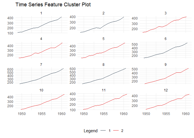

#> 
#> $plot$plotly_plot
#> 
#> 
#> $data
#> $data$original_data
#> # A tibble: 144 × 4
#>    index     date_col   value group_id
#>    <yearmon> <date>     <dbl>    <int>
#>  1 Jan 1949  1949-01-01   112        1
#>  2 Feb 1949  1949-02-01   118        2
#>  3 Mar 1949  1949-03-01   132        3
#>  4 Apr 1949  1949-04-01   129        4
#>  5 May 1949  1949-05-01   121        5
#>  6 Jun 1949  1949-06-01   135        6
#>  7 Jul 1949  1949-07-01   148        7
#>  8 Aug 1949  1949-08-01   148        8
#>  9 Sep 1949  1949-09-01   136        9
#> 10 Oct 1949  1949-10-01   119       10
#> # ℹ 134 more rows
#> 
#> $data$kmm_data_tbl
#> # A tibble: 3 × 3
#>   centers k_means  glance          
#>     <int> <list>   <list>          
#> 1       1 <kmeans> <tibble [1 × 4]>
#> 2       2 <kmeans> <tibble [1 × 4]>
#> 3       3 <kmeans> <tibble [1 × 4]>
#> 
#> $data$user_item_tbl
#> # A tibble: 12 × 8
#>    group_id ts_x_acf1 ts_x_acf10 ts_diff1_acf1 ts_diff1_acf10 ts_diff2_acf1
#>       <int>     <dbl>      <dbl>         <dbl>          <dbl>         <dbl>
#>  1        1     0.741       1.55       -0.0995          0.474       -0.182 
#>  2        2     0.730       1.50       -0.0155          0.654       -0.147 
#>  3        3     0.766       1.62       -0.471           0.562       -0.620 
#>  4        4     0.715       1.46       -0.253           0.457       -0.555 
#>  5        5     0.730       1.48       -0.372           0.417       -0.649 
#>  6        6     0.751       1.61        0.122           0.646        0.0506
#>  7        7     0.745       1.58        0.260           0.236       -0.303 
#>  8        8     0.761       1.60        0.319           0.419       -0.319 
#>  9        9     0.747       1.59       -0.235           0.191       -0.650 
#> 10       10     0.732       1.50       -0.0371          0.269       -0.510 
#> 11       11     0.746       1.54       -0.310           0.357       -0.556 
#> 12       12     0.735       1.51       -0.360           0.294       -0.601 
#> # ℹ 2 more variables: ts_seas_acf1 <dbl>, ts_entropy <dbl>
#> 
#> $data$cluster_tbl
#> # A tibble: 12 × 9
#>    cluster group_id ts_x_acf1 ts_x_acf10 ts_diff1_acf1 ts_diff1_acf10
#>      <int>    <int>     <dbl>      <dbl>         <dbl>          <dbl>
#>  1       2        1     0.741       1.55       -0.0995          0.474
#>  2       2        2     0.730       1.50       -0.0155          0.654
#>  3       1        3     0.766       1.62       -0.471           0.562
#>  4       1        4     0.715       1.46       -0.253           0.457
#>  5       1        5     0.730       1.48       -0.372           0.417
#>  6       2        6     0.751       1.61        0.122           0.646
#>  7       2        7     0.745       1.58        0.260           0.236
#>  8       2        8     0.761       1.60        0.319           0.419
#>  9       1        9     0.747       1.59       -0.235           0.191
#> 10       1       10     0.732       1.50       -0.0371          0.269
#> 11       1       11     0.746       1.54       -0.310           0.357
#> 12       1       12     0.735       1.51       -0.360           0.294
#> # ℹ 3 more variables: ts_diff2_acf1 <dbl>, ts_seas_acf1 <dbl>, ts_entropy <dbl>
#> 
#> 
#> $kmeans_object
#> $kmeans_object[[1]]
#> K-means clustering with 2 clusters of sizes 7, 5
#> 
#> Cluster means:
#>   ts_x_acf1 ts_x_acf10 ts_diff1_acf1 ts_diff1_acf10 ts_diff2_acf1 ts_seas_acf1
#> 1 0.7387865   1.528308    -0.2909349      0.3638392    -0.5916245    0.2930543
#> 2 0.7456468   1.568532     0.1172685      0.4858013    -0.1799728    0.2876449
#>   ts_entropy
#> 1  0.6438176
#> 2  0.4918321
#> 
#> Clustering vector:
#>  [1] 2 2 1 1 1 2 2 2 1 1 1 1
#> 
#> Within cluster sum of squares by cluster:
#> [1] 0.3660630 0.3704304
#>  (between_SS / total_SS =  59.8 %)
#> 
#> Available components:
#> 
#> [1] "cluster"      "centers"      "totss"        "withinss"     "tot.withinss"
#> [6] "betweenss"    "size"         "iter"         "ifault"

Event Analysis

Analyze time series behavior before and after significant events (e.g., policy changes, new treatments):

library(dplyr)
df <- ts_to_tbl(AirPassengers) %>% select(-index)

ts_time_event_analysis_tbl(
  .data = df,
  .horizon = 6,
  .date_col = date_col,
  .value_col = value,
  .direction = "both"
) %>%
  ts_event_analysis_plot()



ts_time_event_analysis_tbl(
  .data = df,
  .horizon = 6,
  .date_col = date_col,
  .value_col = value,
  .direction = "both"
) %>%
  ts_event_analysis_plot(.plot_type = "individual")

ARIMA Simulation

Generate realistic ARIMA time series for testing and validation:

output <- ts_arima_simulator()
output$plots$static_plot

Available Models

Automated Workflow Functions

Each function creates a complete modeling pipeline including recipe, model specification, workflow, fitting, and calibration:

Function	Model Type	Description
`ts_auto_arima()`	ARIMA	Automatic ARIMA with auto-tuning
`ts_auto_arima_xgboost()`	Hybrid	ARIMA errors with XGBoost
`ts_auto_prophet_reg()`	Prophet	Facebook’s Prophet algorithm
`ts_auto_prophet_boost()`	Hybrid	Prophet with XGBoost
`ts_auto_xgboost()`	ML	Gradient boosting
`ts_auto_nnetar()`	Neural Net	Neural network autoregression
`ts_auto_exp_smoothing()`	ETS	Exponential smoothing
`ts_auto_smooth_es()`	Smooth	Smooth package ETS
`ts_auto_theta()`	Theta	Theta method
`ts_auto_croston()`	Croston	For intermittent demand
`ts_auto_lm()`	Linear	Linear regression with time features
`ts_auto_mars()`	MARS	Multivariate adaptive regression splines
`ts_auto_glmnet()`	GLM	Elastic net regression
`ts_auto_svm_poly()`	SVM	Support vector machine (polynomial)
`ts_auto_svm_rbf()`	SVM	Support vector machine (radial)

Function Categories

healthyR.ts includes 90+ functions organized into these categories:

📊 Data Generators: Create synthetic time series data (random walks, Brownian motion, ARIMA)
📈 Plotting Functions: Comprehensive visualization suite for time series
🔍 Clustering: Feature-based time series clustering and analysis
🤖 Forecasting: Automated modeling workflows and model comparison
📐 Statistical Functions: Tests, transformations, and time series statistics
🔧 Utilities: Helper functions for data manipulation and transformation
📉 Augment Functions: Add features like velocity, acceleration, and growth rates
🧮 Vector Functions: Vectorized operations for time series
🔬 Recipe Steps: Custom tidymodels recipe steps for time series

Documentation

📘 Getting Started Vignette - Comprehensive introduction
📗 Function Reference - Complete function documentation
📙 Package Website - Full documentation site
📕 News/Changelog - Version history and updates

Learning Resources

Vignettes

Example Use Cases

Hospital Admissions Forecasting - Predict daily/weekly admissions using multiple models
Length of Stay Analysis - Analyze and forecast ALOS trends
Readmission Rate Monitoring - Track and predict readmission patterns
Resource Planning - Forecast bed occupancy and staffing needs
Seasonal Pattern Detection - Identify and visualize seasonal trends in clinical data

Contributing

Contributions are welcome! Here’s how you can help:

🐛 Report bugs via GitHub Issues
💡 Suggest features through issue requests
🔧 Submit pull requests for bug fixes or new features
📖 Improve documentation by suggesting clarifications or additions

Please follow the tidyverse style guide for code contributions.

healthyR - Hospital data analysis companion package
healthyR.ai - Machine learning companion for healthcare
healthyverse - Meta-package loading all healthyR packages

Citation

If you use healthyR.ts in your research or publications, please cite:

citation("healthyR.ts")

Support

📧 Email: spsanderson@gmail.com
🐦 Issues: GitHub Issue Tracker
🌐 Website: https://www.spsanderson.com/healthyR.ts/